2 · Vision models#
How an image becomes a vector, and the three tricks used to make that vector useful: self-supervision, contrastive learning, and generative vision–language models.
1. An image becomes a vector#
Explanation. An encoder is a neural network that turns an image into a fixed-length vector, called a feature or embedding. "Frozen" means the encoder's weights are not changed during your task. A classifier on top then maps the vector to a label.
Term. Linear probe: a single layer \(p = \mathrm{softmax}(Wz+b)\) trained on fixed features \(z\). Fine-tuning updates the encoder itself.
Check yourself
Encoder A gets 78% with a frozen linear probe and 86% fine-tuned; B gets 84% and 85%. Which encoder do you pick in each case, and what does the table not prove?
Answer
Frozen: B (84 > 78). Fine-tuned: A (86 > 85). A probe measures only how linearly separable the existing features are; fine-tuning can reshape them, so A may be less linearly accessible but more adaptable. The table does not establish significance (one split, no intervals), external validity, overfitting, or cost — a one-point gap is within noise.
2. Self-supervised learning makes its own labels#
Explanation. Self-supervised means the supervision comes from the data itself, not from annotators. One recipe: take two augmented views of the same image (crop, colour jitter, blur), and train the model to give them similar representations. It learns invariance — the representation ignores changes that do not change the content.
Check yourself
Why do two different views of the same image help a model learn without labels, and what can augmentation accidentally destroy?
Answer
The two views are related observations of the same content, so forcing consistent representations teaches invariance to irrelevant changes. Aggressive augmentation can destroy clinically meaningful detail (a small lesion cropped away), which is why medical self-supervision uses gentler transforms.
3. DINO: a student learns from a slow teacher#
Explanation. DINO passes two views through a student network and a teacher network. The teacher's output is the target; the student is trained to match it. The teacher's weights are an exponential moving average (EMA) of the student's: $ \theta_\text{teacher} \leftarrow m\,\theta_\text{teacher} + (1-m)\,\theta_\text{student}$. The momentum \(m\) controls how slowly the teacher changes.
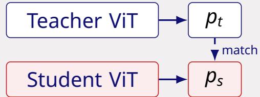
The student sees one crop and must predict what the teacher sees in another. The teacher is a slow copy of the student, so the targets stay stable.
Check yourself
Compare \(m = 0\), \(0.9\), \(0.999\) and \(1\). Why does a slowly changing teacher help?
Answer
\(m=0\): teacher = student, the target moves every step and training can oscillate or collapse. \(0.9\): memory of ~10 steps, only mild stability. \(0.999\): memory of ~1000 steps, stable targets that prevent collapse — the useful regime. \(m=1\): frozen random teacher, stable but useless because the student learns meaningless initial features. A slow teacher acts like an ensemble of past students, giving low-variance targets.
4. Collapse: when all images look the same#
Explanation. A trivial way to make two views similar is to output the same vector for every image — representation collapse. DINO avoids it with centring (subtract the batch mean from the teacher's outputs, so no single dimension dominates) and sharpening (divide the logits by a small temperature, making the target distribution confident); DINOv2 adds a feature-spread regulariser that pushes features apart (prevents dimensional collapse, where features crowd into a narrow subspace).
Check yourself
Remove the spread regulariser. What goes wrong, and which measurements would reveal it?
Answer
Features crowd into a narrow region: neighbours become uninformative and patch features lose the diversity needed for segmentation, even if total collapse is avoided. Reveal it with the effective rank of the feature matrix, pairwise and kNN distance distributions, linear-probe accuracy, patch-level probes and clustering quality — the matching loss alone can look fine.
5. CLIP: match images with text#
Explanation. CLIP trains an image encoder and a text encoder together. For a batch of \(N\) image–text pairs it maximises the similarity of the \(N\) correct pairs and minimises the \(N^2-N\) wrong ones — a contrastive objective. Afterwards, zero-shot classification compares an image with the embeddings of candidate text prompts.
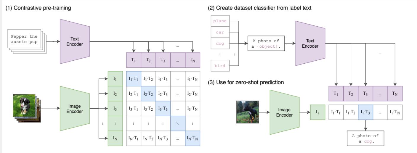
The diagonal is correct pairs; everything off the diagonal is pushed apart. At test time the text side becomes a list of prompts.
Check yourself
A batch contains two different images paired with the same caption. Can each image put all probability on its own copy, and how do you fix it?
Answer
No. Both texts are identical, so their similarities to a given image are equal; the softmax cannot give all mass to one copy and none to the other, and the gradients conflict. Fix by deduplicating the batch, ensuring unique texts, or using a multiple-positive contrastive loss that treats all identical texts as positives.
6. A softmax over prompts is not a probability#
Explanation. CLIP computes a similarity for each candidate prompt and applies softmax over that candidate set. Adding a prompt changes the denominator, so every score changes even if the image is untouched. The output is a relative ranking among the prompts you wrote, not a calibrated disease probability.
Check yourself
"Abnormal" scores 0.90 against two prompts. You add a third prompt, "pneumonia", without changing the image. Can the 0.90 change, and is it a 90% chance of disease?
Answer
Yes, it can change: softmax normalises across the candidate set, so a new option takes probability mass from the others. And no — 0.90 is a relative score within that prompt list. A real probability needs calibration on held-out data with a fixed, clinically defined set of classes.
7. Vision–language models need a projection#
Explanation. A VLM such as LLaVA feeds image features into a language model. Vector lengths may match, but the two spaces have different scales and geometry. A learned projection maps image features into the language model's embedding space, and alignment/instruction tuning teaches the model to use those visual tokens (usually several tokens, not one).
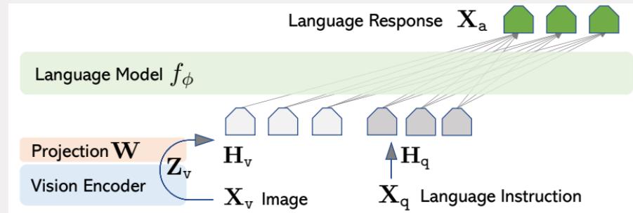
The projection \(W\) is the part that must be trained; without it the language model cannot read the image vector, however well the encoder works.
Check yourself
A frozen CLIP vector has exactly the same dimension as the LLM's token embeddings. Can you feed it in directly?
Answer
No. Same length does not mean same space; the CLIP vector is out of distribution for the LLM, which has never learned to interpret it. You need a trained projection plus alignment training, or the model ignores or misreads the image.
8. Retrieval versus generation#
Explanation. Retrieval selects an existing report from a database by similarity. Generation predicts a new sequence of tokens. Retrieval is grounded and cannot hallucinate a new finding, but it can only reuse what exists; generation is flexible but can fabricate.
Check yourself
For an archive with 200,000 prior reports, which approach would you choose for a first draft, and what is its main failure mode?
Answer
Retrieval: it selects the most similar existing report, so it cannot invent findings, but it can return a report about a different patient or an outdated style/content that does not fit. Generation is more flexible but can hallucinate.
9. Validation decides whether it works#
Explanation. Internal validation holds out part of the same dataset. External validation uses independently collected data from another site, scanner or period. Only external validation tests whether the model transports.
Check yourself
A model has AUROC 0.97 on a random 20% split of one hospital's data. What has been established?
Answer
Internal performance on that hospital's data distribution. Nothing about other scanners, populations or time periods; the split may even leak patients. Transportability requires external validation and, for deployment, local calibration.
If you remember one thing
A CLIP score is a ranking among the prompts you typed, never a disease probability.