How to sit the papers
The written exam is four recycled methods with new numbers. Learn each method on one real question here, then sit two papers under time. The marking keys are at the bottom, after the methods. Do not start by reading the keys.
typical 1.5 / 2.75 / 3 / 2.75
current shape, no key
official key exists
- Practice ordertwo sittings
- Block 1 · probabilityBayes, ACF
- Block 2 · estimationMLE, CRLB, MAP
- Block 3 · spectra~3 of 10 points
- Block 4 · detectionwhich tail
- Marking keysafter you sit
What you walk into
Four exercises, three hours, total 10. Spectra is usually the fattest (about 3 points). After January 2019, every multiple choice has exactly one correct circle, and those questions sit inside all four blocks rather than in a separate Q1. January 2019 was the old style: four MC in Q1, one or two letters allowed, −0.25 per extra wrong letter. Ignore that rule unless you sit that paper.
They grade formulation and order. A correct number with no likelihood written is not full marks. Every year you shade a plot or fill a table in detection, often in spectra too.
Aids: one A4, both sides, typed or handwritten, plus a calculator and a dictionary. The 2026–27 study guide does not promise a provided formula sheet. Write your own; see the A4 page.
| Paper | Why sit it | Key |
|---|---|---|
| Nov 2022 | Current split 1.5 / 2.75 / 3 / 2.75. Closest to what you will get. | none · derived below |
| Jan 2022 resit | Same exam as the Jan 2020 resit, so you can actually mark it. | Resit 2020 solutions |
| Nov 2019 | Correlogram + AR(2) with official numbers. Energy detector. | two keys; 1a conflicts |
| Jan 2020 | The only 5-exercise paper. Least squares / Gauss–Newton live here. | oldexams |
| Practice Oct 2021 | Virus Bayes (37%). ARMA(1,1) with \(r[0]=28/27\). PMFs printed on the sheet. | Q&A slides; 1f missing |
| Jan 2019 retake | erf table. Exponential MLE. 2-tap Wiener is legacy: skip Q4 as a model of 2026. | oldexams |
Do not count the 2020 resit and the 2022 resit as two different papers. They are the same exam. Practice Q3 is also SLT6 2025–26 question 6.2. January 2019 Q3 is SLT7 7.1.
Practice order
- Read the four block walkthroughs on this page. Close the spoilers. Do not open the marking keys yet.
- Sit November 2022 in three hours with only the A4 and a calculator. There is no official key, so you cannot mark letters from a sheet. After the clock, compare to the derived column and treat those as derived.
- Sit January 2022 resit in three hours. Grade with the official key. This is the paper that tells you if the methods stuck.
- If you want more reps: November 2019 (two keys, question 1a fights) or January 2020 (least squares). Stop there. Seven papers of grinding without the methods does nothing.
Write the likelihood, the Yule–Walker 2×2, and the inequality direction of the LRT on the script. Those three lines are what they mark, not the final boxed number alone.
Block 1 · they swapped the condition
Notation for this block
Every Block-1 Bayes question uses the same five objects. Write them down before you touch a number:
| Object | Symbol | Example (virus question) |
|---|---|---|
| Observation | \(A\) | test is positive |
| Hidden cause | \(B\) | person is infected |
| Prior | \(P(B)\) | 1.8% infected, before any test |
| Likelihood | \(P(A\mid B)\) | 95% sensitivity |
| Evidence | \(P(A)\) | positives overall — the denominator |
Reading rules. \(P(A\mid B)\) is "probability of \(A\) given \(B\)" — the bar means "given", the right side is what you assume true. \(B^c\) means "not \(B\)". The two conditionals \(P(A\mid B)\) and \(P(B\mid A)\) run in opposite directions and are different numbers: the first is what the test manufacturer prints, the second is what the doctor wants. Bayes turns one into the other. Swapping them is the exam.
Bayes, with the complement in the denominator
You are given how the data look if a cause is true (sensitivity, pass rate of a machine). You are asked how likely the cause is, given the data. Those are not the same number. Bayes unswaps them. The distractors are always the sensitivity, or \(P(\text{data})\) with no cause.
Method, every time — write these four lines on the script:
- Name. One line: "let \(A =\) [what you observed], \(B =\) [hidden cause]".
- List. Prior \(P(B)\); likelihood \(P(A\mid B)\); false-positive rate \(P(A\mid B^c)\). Translate words to symbols first — half the errors happen here, not in the arithmetic.
- Denominator. Total probability: the data happen with the cause plus without it. Both terms. This line alone is often worth 1 pt (machines Q2a, Nov22 1a).
- Divide. Numerator = the "with the cause" pile; denominator = everything.
Distractor map: the option equal to the sensitivity skipped the denominator. The option equal to the prior ignored the test. If your answer equals either printed number, you fell for it.
Practice exam · 28 Oct 2021 · 1a · 0.5 pt · one correct
A virus has infected 1.8% of a population. A test detects this virus 95% of the time when it is actually present, but it returns a false positive 3% of the time when the virus is not present. If a person selected at random from this population tests positive for the virus, what is the probability that this person is actually infected? Please round to the nearest percent.
- a) 26%
- b) 37%
- c) 95%
- d) 92%
Step 1 — name. \(A =\) "tests positive" (observed). \(B =\) "infected" (hidden). You want \(P(B\mid A)\), not \(P(A\mid B)\).
Step 2 — list. "Infected 1.8%" is the prior: \(P(B)=0.018\), so \(P(B^c)=0.982\). "Detects 95% when present" is the sensitivity: \(P(A\mid B)=0.95\). "False positive 3% when not present": \(P(A\mid B^c)=0.03\). Note the 95% and the 3% condition on opposite causes — they live on different rows, never add them.
Step 3 — denominator. Positives come from two piles:
$$ P(A)=\underbrace{0.95\cdot 0.018}_{\text{sick, detected}}+\underbrace{0.03\cdot 0.982}_{\text{healthy, false alarm}}=0.0171+0.02946=0.04656. $$Step 4 — divide.
$$ P(B\mid A)=\frac{0.0171}{0.04656}\approx 0.367. $$Official: b) 37%. Option c is the sensitivity \(P(A\mid B)\) — step 2 without steps 3–4. Sanity in people, not decimals: in 10 000 people, about 180 are infected and 171 of those test positive. About 9 820 are healthy and 295 of those still test positive. Most of the positives are healthy — rare disease, noisy test, the false-positive pile wins. Whenever the prior is tiny, expect the posterior far below the sensitivity.
Written exam · 20 Jan 2020 · Q2 · 2 pt
A car production company has three machines \(M_1\), \(M_2\), and \(M_3\) for painting cars. It has been observed that 85% of the cars painted by \(M_1\) pass the quality test, while for machines \(M_2\) and \(M_3\) the percentages of a car passing the quality test are 92% and 60%, respectively. Each day, machine \(M_1\) paints 30 cars, \(M_2\) paints 45 cars, and \(M_3\) paints 25 cars. All the cars are mixed at random before quality control.
- (a) What is the probability that a car will pass the quality test? [1 pt]
- (b) What is the probability that a car that has passed the test was painted by machine \(M_3\)? [1 pt]
Step 1 — name. \(A =\) "passes". Causes \(M_1,M_2,M_3\) (three, not two — the denominator gets three terms).
Step 2 — priors from counts. 30 + 45 + 25 = 100 cars a day, so \(P(M_1)=0.30\), \(P(M_2)=0.45\), \(P(M_3)=0.25\). Likelihoods: \(P(A\mid M_1)=0.85\), \(P(A\mid M_2)=0.92\), \(P(A\mid M_3)=0.60\). ("85% of cars painted by M1 pass" conditions on the machine: \(P(A\mid M_1)\), not \(P(M_1\mid A)\).)
(a) is step 3 of the method — total probability:
$$P(A)=0.30\cdot 0.85+0.45\cdot 0.92+0.25\cdot 0.60=0.255+0.414+0.150=0.819.$$(b) is step 4 — and it reuses (a). Never recompute the denominator:
$$P(M_3\mid A)=\frac{0.25\cdot 0.60}{0.819}=\frac{0.150}{0.819}\approx 0.18.$$Official: \(0.819\) and \(0.18\). Exam tactic: (a) and (b) are one Bayes split across two subparts — (b) without (a) is impossible, so if you blank on (a), write the denominator formula anyway for method marks.
Resit · 24 Jan 2022 (same as resit 24 Jan 2020) · 1a · 0.3 pt · one correct
A small manufacturing company has rated 75% of its employees as satisfactory (\(S\)) and 25% as unsatisfactory (\(S^c\)). Personnel records show that 80% of the satisfactory workers had previous work experience (\(E\)) in the job they are now doing, while 15% of the unsatisfactory workers had no work experience (\(E^c\)) in the job they are now doing. If a person who has had previous work experience is hired, what is the approximate empirical probability that this person will be an unsatisfactory employee?
- a) 0.24
- b) 0.25
- c) 0.26
- d) 0.28
Step 1 — name. Observed \(E =\) "has experience". Hidden \(S^c =\) "unsatisfactory". You want \(P(S^c\mid E)\).
Step 2 — translate, carefully. "80% of satisfactory had experience" is straight: \(P(E\mid S)=0.80\). But "15% of unsatisfactory had no experience" is \(P(E^c\mid S^c)=0.15\) — the complement of what the formula needs. Convert immediately:
$$P(E\mid S^c)=1-P(E^c\mid S^c)=1-0.15=0.85.$$Priors: \(P(S)=0.75\), \(P(S^c)=0.25\). Rule: whenever the paper says "had no X" / "did not", flip it to the positive event before listing — plugging 0.15 in as \(P(E\mid S^c)\) is the designed trap.
Steps 3–4.
$$ P(E)=0.80\cdot 0.75+0.85\cdot 0.25=0.600+0.2125=0.8125, \qquad P(S^c\mid E)=\frac{0.85\cdot 0.25}{0.8125}=0.2615\approx 0.26. $$Official: c) 0.26. Option b is the prior \(P(S^c)\) — ignoring the evidence entirely.
Final exam · 7 Nov 2022 · 1a · 0.25 pt · one correct · no official key
About 65% of students who enroll for the exam of the course statistical signal processing have followed the course. Suppose we know that the probability of passing the exam for students who have followed the course is 0.75, while it is 0.4 for students who have not followed it. What is the probability of passing the exam?
- (a) 0.53
- (b) 0.52
- (c) 0.63
- (d) 0.65
This one asks only the denominator — steps 1–3, then stop. \(F =\) followed, \(A =\) pass. \(P(F)=0.65\), \(P(A\mid F)=0.75\), \(P(A\mid F^c)=0.40\):
$$P(A)=0.65\cdot 0.75+0.35\cdot 0.40=0.4875+0.140=0.6275\approx 0.63.$$derived (c) 0.63. Option (d) is the prior \(P(F)\) — no weighting by pass rates. Lesson: some years the whole question is step 3. There is no official key for November 2022; this is the arithmetic of the printed numbers.
Valid ACF, WSS, ergodic, discrete vs continuous
Words first — they are the MC options. A random variable is one number. A random process is a whole waveform per outcome of the experiment. One recording is one realization — one picture is one realization, not the process. Wide-sense stationary (WSS): constant mean, and autocorrelation depending only on the lag, not on absolute time. Ergodic: one infinitely long realization already contains the ensemble — time average equals ensemble average and the variance of that time-average estimator goes to 0. Stationary does not imply ergodic. The lecture counterexample is \(X(t)=A\) with \(A\) random: WSS, but not ergodic in the mean, because each realization is a different flat line and no single line learns the ensemble mean.
Notation. Autocorrelation at lag \(l\): \(r[l]=E[x[n]\,x[n-l]]\). So \(r[0]=E[x^2]\) is the average power, and \(r[1]\) is how much a sample resembles its neighbour. On a stem plot the horizontal axis is the lag \(l\); the center stem (\(l=0\)) is the power.
Three tests, in order, each with its why:
- Even. \(r[-l]=E[x[n]x[n+l]]=r[l]\) — shift the time index and it is the same expectation. For a real process the plot must mirror. No mirror: dead on sight.
- Max at zero. \(|r[l]|\le r[0]\) (Cauchy–Schwarz: a signal resembles a shifted copy of itself at most as much as it resembles itself). The center stem must be the tallest. Any taller side stem: dead.
- Spectrum never negative. \(P(e^{j\theta})=\sum_l r[l]e^{-jl\theta}\ge 0\) — it is power per frequency, and negative power is impossible. Hand check at \(\theta=\pi\): \(e^{-jl\pi}=(-1)^l\), and \(\pm l\) pair up, so \(P(\pi)=r[0]-2r[1]+2r[2]-2r[3]+\cdots\). If that alternating sum is negative: dead.
Apply in order, stop at the first failure — that is the fastest path through six options.
Written exam · 20 Jan 2020 · 1a · 0.25 pt · one correct
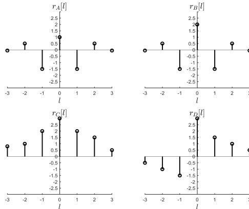
Looking at Figure 1, which sequences are legitimate auto-correlation functions?
- A. Only \(r_B[l]\).
- B. Only \(r_D[l]\).
- C. \(r_A[l]\) and \(r_B[l]\).
- D. \(r_B[l]\) and \(r_D[l]\).
- E. \(r_C[l]\) and \(r_D[l]\).
- F. All.
\(r_D\): fails test 1. Not a mirror — invalid before any arithmetic. That kills B, D, E immediately.
\(r_A\): passes test 1, fails test 2. Even, but a side stem is taller than the center (\(|r[1]|>r[0]\)). This is the option that punishes "even is enough" — checking the mirror and stopping. That kills C and F.
\(r_C\): passes tests 1–2, fails test 3. Even, center tallest — so the first two tests say yes. Read the stems (\(r[0]=2.5\), \(r[1]=2\), \(r[2]=1\), \(r[3]=0.5\)) and run the \(\theta=\pi\) check:
$$P(\pi)=2.5-2\cdot 2+2\cdot 1-2\cdot 0.5=2.5-4+2-1=-0.5<0.$$Negative power: impossible, not a valid ACF. This is the option that punishes "two tests are enough".
\(r_B\): passes all three. Only survivor. Official: A. What to write: one line per candidate naming the test it fails — that is the full answer.
Retake · 21 Jan 2019 · 1a · 0.5 pt · one or two correct
Let \(X\) be a random variable. Which \(X\) defined below is discrete?
- A. Take a random student in the classroom and let \(X\) be his/her weight.
- B. Roll the dice \(n\) times and let \(X\) be the number of 4s.
- C. Take a person in the street and let \(X\) be his/her phone number.
- D. Let \(X\) be the time it takes for you to get to university in the morning.
Rule. Discrete = the values form a countable list (each outcome has its own probability bar). Continuous = any value in an interval (only intervals have probability). Weight (A) and commute time (D) are intervals: continuous. Count of fours (B) is \(0,1,\dots,n\): discrete.
The trap is C. A phone number looks like a huge integer but it is a label from a finite list of digit strings — countable, so discrete. "Large" is not "continuous". Official: B and C. This paper allowed two letters with −0.25 per extra wrong letter: mark both only if sure of both; a sure single letter beats a guessed pair.
Resit · 24 Jan 2022 · 1b · 0.3 pt · one correct
Suppose we are analyzing a infinite set of pictures. For each pixel in each picture we record its color as an integer between 0 and 255. Which of the following statements is true?
- a) The color of each pixel is a continuous random variable.
- b) Each picture is a realization of a random process, hence a random signal.
- c) The infinite set of pictures represents a wide sense stationary random process.
- d) Each picture represents a random process, and the color of each pixel is a realization of the random process, hence a random signal.
Map the vocabulary first: the process = the whole infinite set with its statistics; one picture = one realization = one random signal. Then kill: (a) 0–255 integers are a finite list → discrete, not continuous. (d) swaps the words — it calls each picture a process. (c) WSS needs a constant mean and lag-only correlation, and nothing in the stem gives you either. Leftover: official b. When a question is pure vocabulary, define the three words first and the options kill themselves.
Resit · 24 Jan 2022 · 1c · 0.3 pt · one correct
Suppose we have infinitely many fair dice and we define a random process as the ensemble of the random signals obtained by rolling each die infinitely many times and recording the number on the upward face. Which of the following statements is true?
- a) This random process is not ergodic, but it is stationary.
- b) This random process is ergodic in the mean and variance.
- c) This random process is ergodic in the mean, but not in the variance.
- d) None of the above.
Fair dice, iid rolls: every single infinite sequence has the same statistics (mean 3.5, same variance) as the ensemble across dice — one realization teaches you everything, so ergodic in mean and variance. Official: b. Memorize the pair, not the letter: iid rolls → ergodic; random constant \(X(t)=A\) → stationary but not ergodic. The exam alternates which one it shows you.
Block 2 · freeze the data, pick \(\theta\)
Notation for this block
| Object | Symbol | Meaning |
|---|---|---|
| Parameter | \(\theta\) (or \(\lambda, A\)) | classical: a fixed unknown number — not random, not a function of the data |
| Data | \(\mathbf{x}=(x_0,\dots,x_{N-1})\) | random: what you observed |
| Likelihood | \(p(\mathbf{x};\theta)\) | the PDF as a function of \(\theta\) with the data frozen. Semicolon = classical, no prior |
| Log-likelihood | \(\ln p(\mathbf{x};\theta)\) | what you differentiate (log is monotone, same maximizer) |
| Score | \(\partial\ln p/\partial\theta\) | its zero is the likelihood equation |
| MLE | \(\hat\theta_{\mathrm{ML}}\) | the \(\theta\) that maximizes the likelihood — a recipe in the data, hence random |
Bar vs semicolon: \(p(\mathbf{x};\theta)\) is classical (no prior exists). \(p(\mathbf{x}\mid\theta)\) is Bayesian (a prior \(p(\theta)\) exists, next section). Same formula, different claim about \(\theta\). Mixing them on the script is a free point lost.
The word "support" means where the PDF is nonzero (e.g. \(x\ge 0\)). If the support moves with \(\theta\) (e.g. \([0,\theta]\)), the maximizer sits on the boundary and the derivative is not zero — look at the function instead. If the support is fixed, differentiate.
Maximum likelihood
You never see \(\theta\). You see noisy data that depend on \(\theta\). Freeze the dataset you actually got. The PDF as a function of \(\theta\) is the likelihood. Pick the \(\theta\) that makes this dataset most plausible.
Method, every time — four lines on the script:
- Joint. IID \(\Rightarrow\) product: \(p(\mathbf{x};\theta)=\prod_n p(x_n;\theta)\). Write it — they mark formulation.
- Log. Product \(\Rightarrow\) sum. Drop constants that do not depend on \(\theta\).
- Score = 0. Differentiate in \(\theta\) (the data are frozen numbers), set to 0, solve.
- Max check. Second derivative < 0 (interior max), or boundary argument if the support moves with \(\theta\).
Sanity per family: a rate is one over a mean time (\(\lambda=1/\bar x\)); a scale of \(x^2\) comes with a square root. If your answer has the wrong shape, re-derive — do not box it.
Retake · 21 Jan 2019 · 2a · 1 pt
For the random variable \(x\) with distribution
$$p(x;\lambda)=\lambda e^{-\lambda x}$$find the maximum likelihood estimator for \(\lambda\), given \(N\) independent identically distributed observations \(x_i\), \(i\in\{0:N-1\}\).
Step 1 — joint. IID, so the joint is a product. Each sample contributes one \(\lambda e^{-\lambda x_i}\):
$$p(\mathbf{x};\lambda)=\prod_{i=0}^{N-1}\lambda e^{-\lambda x_i}=\lambda^N\exp\Big(-\lambda\sum_{i=0}^{N-1}x_i\Big).$$Step 2 — log. Products become sums. Drop nothing yet (both terms depend on \(\lambda\)):
$$\ln p(\mathbf{x};\lambda)=N\ln\lambda-\lambda\sum_i x_i.$$Step 3 — score = 0. Differentiate in \(\lambda\) (the data \(\sum x_i\) is a frozen number here):
$$\frac{\partial}{\partial\lambda}\ln p=\frac{N}{\lambda}-\sum_i x_i\stackrel{!}{=}0 \qquad\Rightarrow\qquad \hat\lambda_{\mathrm{ML}}=\frac{N}{\sum_i x_i}=\frac{1}{\bar x}.$$Step 4 — max check. Second derivative \(-N/\lambda^2<0\), so it is a maximum, and it is interior (\(\lambda>0\), support \(x\ge 0\) does not move with \(\lambda\)).
Official: that formula. Sanity holds (rate = 1/mean). For finite \(N>1\) it is biased (\(E[\hat\lambda]=N\lambda/(N-1)\), because \(1/\sum x_i\) is inverse-gamma) — they still want the MLE, not the unbiased cousin \((N-1)/\sum x_i\). What loses the point here is writing the joint as a sum, or differentiating \(e^{-\lambda x}\) without the \(N\ln\lambda\) term.
Written exam · 4 Nov 2019 · 3a · 1 pt
The data \(x[0],x[1],\dots,x[N-1]\) are observed, where \(x[n]\)’s are independent and identically distributed according to the PDF
$$p(x;\theta)=\frac{x}{\theta^2}\exp\left[-\frac{x^2}{2\theta^2}\right],\qquad x\ge 0.$$Find the maximum likelihood estimator for the parameter \(\theta\).
Step 1–2 — log-likelihood, term by term. Take \(\ln\) of one sample: \(\ln x-2\ln\theta-x^2/(2\theta^2)\). Sum over \(N\) iid samples. The \(\sum\ln x[n]\) pile does not depend on \(\theta\) so it dies on differentiation — but write it, they mark formulation:
$$\ln p(\mathbf{x};\theta)=\sum_{n=0}^{N-1}\ln x[n]-2N\ln\theta-\frac{1}{2\theta^2}\sum_{n=0}^{N-1}x^2[n].$$Step 3 — score. Differentiate in \(\theta\) (watch the chain rule on \(1/\theta^2\)):
$$\frac{\partial}{\partial\theta}\ln p=-\frac{2N}{\theta}+\frac{1}{\theta^3}\sum_n x^2[n]\stackrel{!}{=}0.$$Solve. Multiply by \(\theta^3\) (\(\theta>0\)): \(-2N\theta^2+\sum x^2[n]=0\), so
$$\hat\theta_{\mathrm{ML}}=\sqrt{\frac{1}{2N}\sum_{n=0}^{N-1}x^2[n]}.$$Step 4. Keep the positive root (\(\theta>0\) is a scale). Second derivative at the solution is negative — interior max, support \(x\ge 0\) fixed.
Official: that square root. Sanity holds (\(\theta^2\) sits under a mean square). Now the cousin below — same family, different parametrization. Read the exponent before you copy last year's answer.
Practice exam · 28 Oct 2021 · 2b · 1 pt
For the data vector \(\mathbf x\) consisting of independent samples with probability density function
$$p(x[n])=\frac{x}{\theta}\exp\left(-\frac{x^2}{2\theta}\right),\qquad n=0,1,\dots,N-1,$$find an estimator for the parameter \(\theta\).
Compare with 2019 first. There: \(\theta^2\) in the denominator and in the exponent. Here: bare \(\theta\) in both. Same three steps — joint, \(\ln\), score:
$$\ln p=\sum\ln x[n]-N\ln\theta-\frac{1}{2\theta}\sum x^2[n],\qquad -\frac{N}{\theta}+\frac{\sum x^2[n]}{2\theta^2}=0,$$so official MLE \(\hat\theta=(1/(2N))\sum x^2[n]\), no square root. If you memorised "Rayleigh → square root" you lose this point: the exam deliberately re-parametrises the same family to test whether you derive or recall. Side effect for the CRLB: \(\mathbb{E}[x^2]=2\theta\) here vs \(2\theta^2\) in the 2019 version — different Fisher, different bound.
Final exam · 7 Nov 2022 · 2d · 0.5 pt · no official key
Consider the observation
$$\mathbf x=A\begin{bmatrix}\cos\theta\\\sin\theta\end{bmatrix}+\mathbf w,$$where \(\mathbf w\) is white Gaussian noise. The probability density function of the observation is
$$p(\mathbf x;\theta)=\frac{1}{2\pi\sigma^2}\exp\left(-\frac{1}{2\sigma^2}\Big[(x_1-A\cos\theta)^2+(x_2-A\sin\theta)^2\Big]\right).$$Find the maximum likelihood estimator of the parameter \(\theta\).
Step 1 — isolate the \(\theta\) piece. \(A>0\), \(\sigma^2\) known, so the prefactor is a constant. Expand the square:
$$(x_1-A\cos\theta)^2+(x_2-A\sin\theta)^2=x_1^2+x_2^2+A^2-2A(x_1\cos\theta+x_2\sin\theta).$$Only the last term depends on \(\theta\). Maximising the likelihood \(\Leftrightarrow\) minimising that quadratic \(\Leftrightarrow\) maximising \(x_1\cos\theta+x_2\sin\theta\). Everything else is a constant — cross it out mentally.
Step 2 — phasor form. Any \(a\cos\theta+b\sin\theta\) is \(R\cos(\theta-\phi)\) with \(R=\sqrt{a^2+b^2}\), \(\phi=\mathrm{atan2}(b,a)\). Here \(a=x_1\), \(b=x_2\):
$$x_1\cos\theta+x_2\sin\theta=R\cos(\theta-\phi),\qquad R=\sqrt{x_1^2+x_2^2},\ \phi=\mathrm{atan2}(x_2,x_1).$$Step 3 — peak. \(\cos\) peaks at 0, so \(\hat\theta_{\mathrm{ML}}=\phi=\mathrm{atan2}(x_2,x_1)\). derived
Trap — why not \(\arctan\). Setting \(\partial/\partial\theta=0\) gives \(\tan\theta=x_2/x_1\), which has two solutions \(\phi\) and \(\phi+\pi\) (max and min). \(\arctan(x_2/x_1)\) returns one number in \((-\pi/2,\pi/2]\) and loses the quadrant: e.g. \((x_1,x_2)=(-1,-1)\) is angle \(-3\pi/4\), but \(\arctan(1)=\pi/4\) — off by \(\pi\). Two-argument \(\mathrm{atan2}\) keeps the signs of \(x_1,x_2\). On the script, the \(R\cos(\theta-\phi)\) line is the line they mark; it proves you picked the max, not just a stationary point.
Resit · 24 Jan 2022 · 2b · 0.3 pt · one correct
Which of the following statements about the maximum likelihood estimator is true?
- (a) The maximum likelihood estimate is the value of \(x\) that maximizes the likelihood function.
- (b) For large sample sizes, the maximum likelihood estimate is uniformly distributed, i.e. \(\hat\theta_{\mathrm{ML}}\sim\mathrm{Uniform}(-a,a)\) where \(a=\mathcal I^{-1}(\theta)\).
- (c) For a transformed parameter \(\alpha=\psi(\theta)\), where \(\psi(\cdot)\) is a one-to-one mapping, the maximum likelihood estimate \(\hat\theta_{\mathrm{ML}}\) can be obtained as \(\hat\theta_{\mathrm{ML}}=\psi^{-1}(\hat\alpha_{\mathrm{ML}})\) where \(\psi^{-1}(\cdot)\) is the inverse mapping of \(\psi(\cdot)\) and \(\hat\alpha_{\mathrm{ML}}\) is the maximum likelihood estimate of the transformed parameter \(\alpha\), respectively.
Three claims, three verdicts. (a) maximises in the wrong variable: the likelihood is maximised over \(\theta\) with the data frozen, not over \(x\). (b) wrong law: asymptotically the MLE is Gaussian \(\mathcal{N}(\theta,\mathcal{I}^{-1})\), not uniform. (c) is invariance — maximise in the convenient parametrization, then transform. Official: c. Invariance in one sentence: if \(\alpha=e^A\) and \(\hat A=\bar x\), then \(\hat\alpha=e^{\bar x}\) with no new likelihood needed.
Fisher information and the CRLB
Notation. Fisher information \(\mathcal{I}(\theta)\) is the expected curvature of the log-likelihood — how sharply the likelihood peaks at the truth. Sharp peak = informative data = low bound. Two forms, same number:
$$\mathcal{I}(\theta)=\mathbb{E}\left[\left(\frac{\partial\ln p}{\partial\theta}\right)^2\right]=-\mathbb{E}\left[\frac{\partial^2\ln p}{\partial\theta^2}\right].$$The second is almost always easier: differentiate twice, take expectation, flip sign. \(\mathcal{I}(\theta)\ge 0\) — Fisher is a positive number. (The expected second derivative itself is negative; the 2022 2a trap calls Fisher "strictly negative".) The Cramér–Rao bound: every unbiased estimator has
$$\mathrm{Var}[\hat\theta]\ge\frac{1}{\mathcal{I}(\theta)}\qquad\text{(not }\ge\mathcal{I}\text{ — the reciprocal).}$$For \(N\) iid samples Fisher adds: \(\mathcal{I}_N=N\cdot i(\theta)\), so the bound shrinks as \(1/N\). An unbiased estimator that attains the bound is efficient, hence the MVUE. The attainment test is the identity \(\partial\ln p/\partial\theta=\mathcal{I}(\theta)(g(\mathbf{x})-\theta)\): if the score factors that way, \(g\) is efficient; if not, no finite-sample efficient estimator exists (you still quote the bound).
Regularity — read before grinding. The proof passes \(d/d\theta\) under the integral, which needs the support fixed. If you see \(x\in[0,\theta]\) or \(x\ge\theta\): stop. No CRLB, MLE is \(\max\)/\(\min\) on the boundary (previous section's uniform). Writing Fisher there earns zero.
Resit · 24 Jan 2022 · 2a · 0.3 pt · one correct
Which of the following statements about the Cramer Rao lower bound is true?
- (a) The Cramer Rao lower bound can always be derived.
- (b) For identical and independent distributed observations, the Cramer Rao lower bound decreases linearly with the number of observations.
- (c) An estimator whose variance is lower than the Cramer Rao lower bound is called efficient.
(a) is the regularity trap: \([0,\theta]\) support kills the bound (next question). (c) is backwards: efficient means you attain the bound — below it is impossible under regularity. (b): \(\mathcal{I}_N=N\,i\) so the bound is \(1/(Ni)\) — linear in \(1/N\). Official: b.
Resit · 24 Jan 2022 · 2e · 0.5 pt
Let
$$p(x;\theta)=\begin{cases}(2/\theta)\,x,&0\le x\le\theta,\\ 0,&\text{else}\end{cases}$$be the probability density function of an observation \(X\). Check whether or not it is possible to derive the Cramer Rao lower bound. In case it is possible, derive the Cramer Rao lower bound. If it is not possible, justify why.
Step 1 — look at the support, not the formula. The PDF lives on \([0,\theta]\) — the upper limit is the parameter. Regularity fails: \(d/d\theta\int_0^\theta\neq\int_0^\theta\partial/\partial\theta\) (Leibniz leaves boundary terms). Step 2 — write the one sentence. Official: "cannot — the domain of integration depends on \(\theta\), regularity violated." That sentence is the full 0.5 pt; any Fisher computation after it earns nothing. Same trap as \(\mathrm{Unif}[0,\theta]\) (MLE \(=\max_i x_i\), boundary, no derivative).
Written exam · 4 Nov 2019 · 3b · 1 pt
Same PDF as 3a above,
$$p(x;\theta)=\frac{x}{\theta^2}\exp\left[-\frac{x^2}{2\theta^2}\right],\qquad x\ge 0.$$Find the Cramer-Rao Lower Bound for the MLE.
Step 0 — regularity passes (support \(x\ge 0\) fixed), so proceed. Step 1 — second derivative. From 3a, score \(-2N/\theta+(1/\theta^3)\sum x^2[n]\). Differentiate again:
$$\frac{\partial^2}{\partial\theta^2}\ln p=\frac{2N}{\theta^2}-\frac{3}{\theta^4}\sum_n x^2[n].$$Step 2 — expectation. Fisher is \(-\mathbb{E}[\cdot]\). You need \(\mathbb{E}[x^2]\): either integrate \(\int_0^\infty x^2\cdot(x/\theta^2)e^{-x^2/(2\theta^2)}dx=2\theta^2\), or notice \(x/\theta\) is standard Rayleigh (scale 1), whose second moment is 2. So \(\mathbb{E}[\sum x^2]=N\cdot 2\theta^2\):
$$\mathcal{I}(\theta)=-\frac{2N}{\theta^2}+\frac{3}{\theta^4}\cdot 2N\theta^2=\frac{4N}{\theta^2},\qquad\mathrm{Var}[\hat\theta]\ge\frac{\theta^2}{4N}.$$Notation trap. The published key writes \(\hat\theta^2/(4N)\) — plugged the estimate. The bound is a function of the true parameter (it is the curvature at the truth; you cannot compute it from data). Report \(\theta^2/(4N)\). Efficiency bonus: the score \(-2N/\theta+(1/\theta^3)\sum x^2\) cannot be factored as \(\mathcal{I}(\theta)(g-\theta)\) with \(g\) free of \(\theta\) — so this MLE is not finite-sample efficient, only asymptotically. That one line is how you answer "is it efficient?" anywhere.
MMSE is the mean. MAP is the mode.
Notation shift — the bar appears. Classical: \(\theta\) fixed, \(p(\mathbf{x};\theta)\) with a semicolon. Bayesian: \(\theta\) is drawn from a prior \(p(\theta)\), the same formula becomes a likelihood \(p(\mathbf{x}\mid\theta)\) with a bar, and you update:
$$p(\theta\mid\mathbf{x})=\frac{p(\mathbf{x}\mid\theta)\,p(\theta)}{p(\mathbf{x})}.$$The denominator does not depend on \(\theta\) — drop it for optimisation. From the posterior you return one number. Which one depends on the cost: square cost → posterior mean (MMSE, \(\mathbb{E}[\theta\mid\mathbf{x}]\)); hit-or-miss/uniform cost → posterior mode (MAP, \(\arg\max p(\theta\mid\mathbf{x})\)). Different functions — unless the posterior is symmetric (Gaussian: mean = median = mode, all three coincide).
Method. MMSE: integrate (or sum, if \(\theta\) discrete) \(\theta\) against the posterior. MAP: differentiate \(\ln p(\mathbf{x}\mid\theta)+\ln p(\theta)\); if the unconstrained peak falls outside the prior's support, the max is the boundary (project the MLE onto the support).
Resit · 24 Jan 2022 · 2d · 0.3 pt · one correct
Which of the following statements about the Bayesian estimators is true?
- (a) The minimum mean square error is the maximum of the aposterior PDF.
- (b) The minimum mean square error is the mean of the aposterior PDF.
- (c) The minimum mean square error estimator and the maximum aposterior estimator will always result in a different estimate.
(a) describes MAP (the mode), not MMSE. (c) says "always differ" — one counterexample kills it: a Gaussian posterior has mean = mode. Official: b. ("Aposterior" is the paper's word for posterior.)
Final exam · 7 Nov 2022 · 2f–g · 0.5 + 0.5 pt · no official key
Assume that the parameter \(\theta\ge 0\) is a random variable that admits an exponential distribution with probability density function \(p(\theta)=a e^{-a\theta}\). The conditional probability function of the observation \(x\ge 0\) is \(p(x\mid\theta)=\theta e^{-\theta x}\). Using Bayes’ theorem, the posterior distribution for the parameter \(\theta\) after observing \(x\) is
$$p(\theta\mid x)=\begin{cases}(x+a)^2\theta e^{-(x+a)\theta}&\theta\ge 0,\\ 0,&\text{else.}\end{cases}$$2f. Find the minimum-mean square error estimator. Hint: you can use \(\int x^2 e^{-x}\,dx=-e^{-x}(x^2+2x+2)\).
2g. Find the maximum a posteriori estimator.
Start from the given posterior — do not re-derive Bayes. Recognise the shape: \(b^2\theta e^{-b\theta}\) with \(b=x+a\) is Gamma(shape 2, rate \(b\)). Check the normaliser: \(\int_0^\infty\theta e^{-b\theta}d\theta=1/b^2\) (substitute \(u=b\theta\)), so \(b^2\) makes it a PDF.
2f — MMSE = mean. Gamma mean is shape/rate. Or grind it with the printed hint (\(\int\theta^2 e^{-b\theta}d\theta=2/b^3\) after \(u=b\theta\)):
$$\hat\theta_{\mathrm{MMSE}}=\mathbb{E}[\theta\mid x]=b^2\cdot\frac{2}{b^3}=\frac{2}{b}=\frac{2}{x+a}.$$2g — MAP = mode. \(\ln p(\theta\mid x)=\mathrm{const}+\ln\theta-b\theta\), derivative \(1/\theta-b=0\):
$$\hat\theta_{\mathrm{MAP}}=\frac{1}{x+a}.$$Mode of Gamma(2, \(b\)) is \(1/b\). They differ because the posterior is skewed (long right tail pulls the mean right of the peak) — and that is exactly the 2d-MCQ connection: symmetric posterior → same answer; skewed → different. derived
Resit · 24 Jan 2022 · 2f–h · 0.6 each
Let \(Y=X+N\) where \(X\) and \(N\) are independent random variables. \(X\) takes the values \(+1\) and \(-1\) with equal probability, and \(N\) is a zero-mean Gaussian random variable with variance \(\sigma^2\).
2f. Evaluate the aposteriori probabilities \(P[X=1\mid Y]\) and \(P[X=-1\mid Y]\).
2g. Find the minimum mean square error estimate \(\hat X_{\mathrm{MMSE}}\) of \(X\) given \(Y\). Useful identity printed on the paper:
$$\frac{e^{2u}-1}{e^{2u}+1}=\tanh(u).$$(If 2f failed, the paper prints a garbled fallback for the two posteriors. Use 2f.)
2h. Find the maximum a posterior estimator \(\hat X_{\mathrm{MAP}}\) of \(X\) given \(Y\). More specifically, find a threshold \(y_{\mathrm{th}}\) such that a decision on \(X\) depends on whether or not this threshold is exceeded. Hint: \(X\) is discrete, so \(\hat X_{\mathrm{MAP}}=\arg\max_{X\in\{1,-1\}}P[X\mid Y]\). Check the ratio of the two posteriors.
2f — posteriors. Bayes with equal priors \(P(X=1)=P(X=-1)=1/2\). Likelihoods: \(Y\mid X=1\sim\mathcal{N}(1,\sigma^2)\), \(Y\mid X=-1\sim\mathcal{N}(-1,\sigma^2)\). The 1/2 priors cancel, so each posterior is its likelihood over the sum — a two-class softmax:
$$P[X=1\mid Y=y]=\frac{e^{-(y-1)^2/(2\sigma^2)}}{e^{-(y-1)^2/(2\sigma^2)}+e^{-(y+1)^2/(2\sigma^2)}},$$and symmetrically for \(-1\). (If 2f failed, the paper prints a garbled fallback — trust your 2f, not theirs.)
2g — MMSE = posterior mean, discrete version. \(X\) takes values \(\pm 1\), so the "integral" is a sum: \(\mathbb{E}[X\mid y]=(+1)P_1+(-1)P_{-1}=P_1-P_{-1}\). Divide top and bottom by \(e^{-(y+1)^2/(2\sigma^2)}\); the exponent difference is \((y-1)^2-(y+1)^2=-4y\), so the ratio is \(e^{2y/\sigma^2}\). Then the printed identity with \(u=y/\sigma^2\):
$$\hat X_{\mathrm{MMSE}}=\frac{e^{2y/\sigma^2}-1}{e^{2y/\sigma^2}+1}=\tanh(y/\sigma^2).$$2h — MAP = argmax, threshold. Compare posteriors by their ratio (denominators cancel): \(P_1/P_{-1}=e^{2y/\sigma^2}\gtrless 1\iff y\gtrless 0\). So \(\hat X_{\mathrm{MAP}}=\mathrm{sign}(y)\), threshold \(y_{\mathrm{th}}=0\). Official for both. Read the two against each other: MMSE is soft — a number in \((-1,1)\), near 0 when \(y\approx 0\) ("unsure"), saturating at \(\pm 1\) for large \(|y|/\sigma^2\). MAP is hard — \(\pm 1\), decided at 0. Same sign, different magnitude. That soft-vs-hard contrast is the whole point of asking both.
Retake · 21 Jan 2019 · 2b–c · after the exponential MLE in 2a
Additional information regarding \(\lambda\) is provided in terms of a distribution
$$p(\lambda)=\begin{cases}1/2&0\le\lambda\le 2\\ 0&\text{otherwise.}\end{cases}$$Treat \(p(x;\lambda)\) as a conditional \(p(x\mid\lambda)\). (b) Determine the Bayesian MMSE for \(\lambda\): first write the formula specifying each density, then solve it. (c) Using the same information, find the MAP estimator for \(\lambda\). Integrals \(\int x e^{ax}\,dx\) and \(\int x^2 e^{ax}\,dx\) are printed on the paper.
(c) MAP — project, don't just copy the MLE. The prior is flat (\(1/2\)) on \((0,2)\), so inside that interval maximising the posterior \(\Leftrightarrow\) maximising the likelihood. For one sample, \(\ln p(x\mid\lambda)=\ln\lambda-\lambda x\), score \(1/\lambda-x=0\), unconstrained MLE \(1/x\) (second derivative \(-1/\lambda^2<0\)). Now the boundary: \(\ln\lambda-\lambda x\) is increasing for \(\lambda<1/x\). If \(1/x>2\) (i.e. \(x<1/2\)), it is still increasing on the whole \((0,2]\), so the constrained max is the right endpoint:
$$\hat\lambda_{\mathrm{MAP}}=\begin{cases}2 & x<1/2,\\ 1/x & x\ge 1/2.\end{cases}$$For \(N\) samples the unconstrained MLE is \(N/\sum x_i\); project that onto \([0,2]\). The published key writes only \(N/\sum x_i\) and skips the projection — that answer is MAP only when it already lies in \([0,2]\). (b) MMSE is the posterior mean on \([0,2]\): \(\int_0^2\lambda^2 e^{-x\lambda}d\lambda\big/\int_0^2\lambda e^{-x\lambda}d\lambda\). Closed form in ch. 05-bayes; the published last line has \((x+1)^2\) where \(2x^2+2x+1\) should be. See errata — and note the key answers 2b with a one-sample formula despite \(N\) in 2a.
No noise PDF → least squares
Decision rule — which estimator family. The paper gives a signal model \(s[n]\) but no noise PDF: no \(p(\mathbf{x};\theta)\), so MLE, MAP and BLUE are all off the table (each needs a PDF, or at least a covariance). LS needs only the model: minimise residual energy \(J=\sum(x[n]-s[n])^2\). That choice + the one sentence "requires no function for the noise" (official wording) is the 0.5 pt of (a).
Written exam · 20 Jan 2020 · Q4 · 2.5 pt
Consider the observed data \(x[0],x[1],\dots,x[n]\), which consists of independent identically distributed samples. The data comes from an experiment which generates a signal according to model \(s[n]=A e^{\phi n}\), where the amplitude \(A\) and the power term \(\phi<0\) are to be estimated based on the observed data.
- (a) What kind of estimators can be used to solve this problem? Explain your reasoning and write down the formulations for the estimators that can be used. [0.5 pt]
- (b) For the case where \(\phi\) is known but \(A\) is unknown, find an estimator for \(A\). The estimator you find must have a closed form that depends on \(\phi\) and observed data \(x[0],\dots,x[n]\). [0.5 pt]
- (c) For the case where both \(\phi\) and \(A\) are unknown, write the cost function for an estimator for \(\theta=[\phi\ A]^\top\). Hint: the expression you find will be non-linear, which is why the solution in (d) is asked. [0.5 pt]
- (d) Formulate the Gauss-Newton solution for the estimator cost function derived in (c). Clearly show the iterative formulation. [1 pt]
(b) \(\phi\) known → linear in \(A\). One unknown multiplying a known waveform \(h[n]=e^{\phi n}\). Scalar normal equation \(\hat A=(\mathbf{h}^\top\mathbf{x})/(\mathbf{h}^\top\mathbf{h})\):
$$\hat A_{\mathrm{LS}}=\frac{\sum x[n]e^{\phi n}}{\sum e^{2\phi n}}$$(Key sums \(n=0..N\); match the paper's indexing, not the reader's \(N-1\).)
(c) Both unknown → nonlinear. \(J(\phi,A)=\sum(x[n]-A e^{\phi n})^2\). Nonlinear because \(\phi\) sits inside the exponential — no change of variables linearises both parameters at once. Write the gradient too (it is part d's input): \(\partial J/\partial A=-2\sum e^{\phi n}(x[n]-Ae^{\phi n})\), \(\partial J/\partial\phi=-2\sum Ane^{\phi n}(x[n]-Ae^{\phi n})\).
(d) Gauss–Newton vs what the key printed. Gauss–Newton linearises the signal \(\mathbf{s}(\theta)\) about \(\theta_k=(\phi_k,A_k)\): Jacobian row \(n\) is \([A_k n e^{\phi_k n},\ e^{\phi_k n}]\) (derivatives of \(Ae^{\phi n}\) in \(\phi,A\)), then one linear-LS step \(\theta_{k+1}=\theta_k+(H_k^\top H_k)^{-1}H_k^\top(\mathbf{x}-\mathbf{s}(\theta_k))\). Newton–Raphson instead iterates on \(J\) with its Hessian: \(\theta_{k+1}=\theta_k-(\nabla^2 J)^{-1}\nabla J\). The 2020 key printed the Newton form even though the question said Gauss–Newton. On your script, write the one they name; if they name Gauss–Newton, the Jacobian row is the line they mark. Know both — resit 2022 2c explicitly says both are legal.
Resit · 24 Jan 2022 · 2c · 0.3 pt · one correct
Which of the following statements about the least-squares estimator is true?
- (a) Some nonlinear least-squares estimation problems can be solved analytically by either separating the problem into nonlinear and linear least-squares problems or by transforming the nonlinear problem into a linear problem.
- (b) For linear signal models, the solution vector \(\hat\theta\) is orthogonal to the span of the columns of the observation matrix \(\mathbf H\).
- (c) Only the Gauss-Newton method can be applied for nonlinear least-squares problems but not the Newton-Raphson method.
(b) is the geometry trap — picture it. The columns of \(\mathbf{H}\) span a subspace; the fitted signal \(\hat{\mathbf{s}}=\mathbf{H}\hat\theta\) lies in it. The residual \(\mathbf{x}-\mathbf{H}\hat\theta\) is what sticks out orthogonally — that orthogonality \(\mathbf{H}^\top(\mathbf{x}-\mathbf{H}\hat\theta)=0\) is the normal equation. So \(\hat\theta\) being "orthogonal to the span" is nonsense; the residual is. (c) is false: both Gauss–Newton and Newton–Raphson are legal. Official letter: a (with the 2020 key noting that topic is "no longer part of the content" — Gauss–Newton itself still is).
Block 3 · three curves on \([-\pi,\pi]\)
This is about 3 of 10 points — the fattest block. Typical open part: they hand you an autocorrelation, or a difference equation, or a filter. You draw a correlogram, fit an AR with Yule–Walker, overlay an MA, quote values at \(0\) and \(\pi\). Plus one MC on periodogram / Bartlett / Welch / windows.
Notation for this block
| Object | Symbol | Meaning |
|---|---|---|
| Autocorrelation | \(r[l]=E[x[n]x[n-l]]\) | lag \(l\); \(r[0]=E[x^2]\) is the average power; real processes: \(r[-l]=r[l]\) |
| PSD | \(P(e^{j\theta})\), \(\theta\in[-\pi,\pi]\) | power per frequency; even, non-negative; area\(/2\pi\) = \(r[0]\) |
| Innovation | \(i[n]\), variance \(\sigma_i^2\) | the white drive behind AR/MA/ARMA models |
| AR coeffs | \(a_k\) | course sign: \(x[n]+a_1x[n-1]+\cdots=i[n]\) |
| MA coeffs | \(b_k\) (\(b_0=1\)) | \(x[n]=i[n]+b_1i[n-1]+\cdots\) |
| Yule–Walker | Toeplitz\((r)\) | right-hand side \((\sigma_i^2,0,\dots)^\top\) — not the lags |
Where the cosine sum comes from
The correlogram is the DTFT of the estimated ACF: \(P_{\mathrm{cor}}=\sum_l\hat r[l]e^{-jl\theta}\). For real signals \(\hat r[-k]=\hat r[k]\), so pair lag \(k\) with \(-k\):
$$r[k]e^{-jk\theta}+r[k]e^{+jk\theta}=2r[k]\cos(k\theta).$$The 2 in front of every cosine is the \(\pm k\) pair — not a fudge factor — and \(r[0]\) stands alone. Only lags with nonzero \(r\) enter: a printed zero lag (Nov 2019's \(r[\pm 4]=0\)) contributes nothing. Full form:
$$P_{\mathrm{cor}}(e^{j\theta})=r[0]+2\sum_{k\ge 1}r[k]\cos(k\theta).$$Course AR sign convention — read twice
\(A(z)=1+a_1z^{-1}+\cdots\), difference equation \(x[n]+a_1x[n-1]+\cdots=i[n]\), PSD denominator \(|1+a_1e^{-j\theta}+\cdots|^2\) — the same \(a_1\) everywhere. Minus signs in a PSD come from a negative \(a_1\), never from the formula. Shape read: \(a_1<0\) puts the pole on the positive real axis → low-frequency peak; \(a_1>0\) → high-pass. Cross-check with \(r[1]\): neighbours agree (\(r[1]>0\)) → low-pass; anti-correlated (\(r[1]<0\)) → high-pass. If your sketch and your \(r[1]\) disagree, the sign flipped somewhere.
Yule–Walker in one derivation
Multiply the DE \(x[n]+a_1x[n-1]+\cdots=i[n]\) by \(x[n-l]\) and take \(E\). For \(l\ge 1\), \(E[i[n]x[n-l]]=0\) — today's innovation is independent of past outputs — so \(r[l]+a_1r[l-1]+\cdots=0\). For \(l=0\), \(E[i[n]x[n]]=\sigma_i^2\) — today's innovation is inside today's output — so \(r[0]+a_1r[1]+\cdots=\sigma_i^2\). Stack lags \(0..p\): Toeplitz matrix times \((1,a_1,\dots)^\top\) equals \((\sigma_i^2,0,\dots,0)^\top\). The last \(p\) rows solve the \(a\)'s; the first row then gives \(\sigma_i^2\).
Method — given lags, three curves
- Correlogram: cosine sum. Always quote \(P(0)=r[0]+2\sum r[k]\) (all cosines are 1) and \(P(\pi)=r[0]-2r[1]+2r[2]-\cdots\) (alternating). Even function: compute \([0,\pi]\), mirror. Warning: a truncated ACF need not be a valid ACF, so the curve can go negative — write that sentence, it is the point.
- AR fit: Yule–Walker on lags \(0..p\). PSD \(\sigma_i^2/|A(e^{j\theta})|^2\ge 0\) by construction — strictly positive, sharper peak than the correlogram (the model extrapolates \(r\) past the last given lag instead of truncating it).
- MA fit: finite ACF: \(r[0]=\sigma_i^2(1+b_1^2+\cdots)\), \(r[1]=\sigma_i^2(b_1+b_1b_2+\cdots)\). Quadratic in \(b\) → reciprocal pair → keep \(|b|<1\) (minimum-phase: zero of \(1+bz^{-1}\) at \(z=-b\) inside the unit circle). If the truth is MA(\(q\)), the correlogram of lags \(|l|\le q\) is the MA spectrum — identical curves; an AR fit of the same lags is a different curve.
Method — given \(H(z)\) or a difference equation
Read \(a_k,b_k\) off \(H(z)=B(z)/A(z)\) (watch the signs: \(x=i+b_1i_{-1}-a_1x_{-1}\)). Impulse response: \(h[0]=1\) (direct feedthrough \(i[k]\to x[k]\)), \(h[1]=b_1-a_1\) (one step: \(x[1]=b_1\cdot 1-a_1\cdot 1\)). Modified Yule–Walker at lags 0 and 1 — extra \(b\cdot h\) terms, because recent innovations are inside the current output. For \(|\tau|>q\) the MA part is dead: \(r[\tau]=-a_1r[\tau-1]\) (pure AR tail). Fake AR(1) / MA(1) fits use only \((r[0],r[1])\).
Sketch discipline, every curve: axes \(\theta\in[-\pi,\pi]\), even symmetry, mark \(P(0)\) and \(P(\pi)\). Correlogram may dip below zero; model PSDs may not.
Written exam · 4 Nov 2019 · Q2 · 2 pt
Let \(x[n]\) be a random process whose correlation is estimated. The values for the first five lags are \(r_x[0]=1\), \(r_x[\pm 1]=0.7\), \(r_x[\pm 2]=0.5\), \(r_x[\pm 3]=0.3\), and \(r_x[\pm 4]=0\).
- (a) Determine and plot the correlogram power spectrum estimate. [1 pt]
- (b) Assume that \(x[n]\) is modeled by an AR(2) model. Determine and plot its spectrum estimate. [1 pt]
(a) Correlogram — pair each lag. \(r[\pm 4]=0\) is a distractor: those lags contribute nothing, the sum stops at \(k=3\). Official:
$$P_{\mathrm{cor}}=1+1.4\cos\theta+\cos 2\theta+0.6\cos 3\theta$$Sketch + mandatory numbers. Even on \([-\pi,\pi]\): draw \([0,\pi]\), mirror. At \(\theta=0\) every cosine is 1: \(1+1.4+1+0.6=4\) — always quote this, it is one mark. At \(\theta=\pi\): signs alternate, \(1-1.4+1-0.6=0\). Between them the truncated ACF is not a valid infinite autocorrelation, so the polynomial can go negative (official sketch: small negative sidelobes). Say that on the script — it is the point of the question, not an error in your arithmetic.
(b) AR(2) — Yule–Walker on lags 0,1,2. Unknowns \(a_1,a_2,\sigma_i^2\). Matrix with RHS \((\sigma_i^2,0,0)^\top\) — not the lags:
$$\begin{bmatrix}1&0.7&0.5\\0.7&1&0.7\\0.5&0.7&1\end{bmatrix}\begin{bmatrix}1\\a_1\\a_2\end{bmatrix}=\begin{bmatrix}\sigma_i^2\\0\\0\end{bmatrix}.$$Rows 2–3 are two equations in \(a_1,a_2\): \(0.7+a_1+0.7a_2=0\), \(0.5+0.7a_1+a_2=0\). Eliminate \(a_1\): \(a_2=-0.01/0.51\approx -0.0196\), \(a_1\approx -0.6863\). First row: \(\sigma_i^2=1+0.7a_1+0.5a_2\approx 0.5089\) (official, rounded). So
$$P_{\mathrm{AR2}}=0.5089\big/|1-0.6863 e^{-j\theta}-0.0196 e^{-j2\theta}|^2.$$Sketch vs (a). \(\sigma_i^2/|A|^2\ge 0\) by construction — strictly positive, no negative lobes. Sharper peak at \(\theta=0\) than the correlogram (extrapolates \(r\) past lag 3 instead of truncating). Quote \(P(0),P(\pi)\), label \([-\pi,\pi]\). Sign trap: course PSD denominator is \(|1+a_1e^{-j\theta}+\cdots|^2\) with the same \(a_1\) — here \(a_1\) is negative, hence the minus signs. Flip that sign and the curve inverts.
Written exam · 20 Jan 2020 · Q3 · 2 pt
Let \(x[n]\) be a random process whose auto-correlation is given by
$$r_x[l]=\begin{cases}1/21&l=0\\ 2/105&l=\pm 1\\ 0&\text{else.}\end{cases}$$- (a) Determine and plot the correlogram power spectrum estimate. [0.8 pt]
- (b) Assume that \(x[n]\) can be modeled by an MA(1) random process. Determine and plot its spectrum estimate. How does this relate to the spectrum estimate obtained in 3(a)? Motivate your answer. [1.2 pt]
(a) Correlogram — two lags, one cosine. \(P=r[0]+2r[1]\cos\theta=\frac1{21}+\frac4{105}\cos\theta\). Official. Quote \(P(0)=1/21+4/105=3/35\) and \(P(\pi)=1/21-4/105=1/105\).
(b) MA(1) — solve, then keep min-phase. MA(1) equations: \(r[0]=\sigma_i^2(1+b^2)\), \(r[1]=\sigma_i^2 b\). Divide: \(r[0]/r[1]=(1+b^2)/b\). Here \(r[0]/r[1]=(1/21)/(2/105)=5/2\), so \(b^2-2.5b+1=0\): roots \(b=2\) and \(b=1/2\) — reciprocals, same \(|1+be^{-j\theta}|^2\) up to scale. Uniqueness comes from the innovation filter: causal + stable + minimum-phase means the zero of \(1+bz^{-1}\) (at \(z=-b\)) sits inside the unit circle, forcing \(|b|<1\). Official: \(b=1/2\), \(\sigma_i^2=r[1]/b=4/105\).
The 1.2-pt sentence — relation to (a). A true MA(1) has \(r[k]=0\) for \(|k|>1\), so the correlogram truncated to \(|l|\le 1\) is the MA spectrum: \(\sigma_i^2(1+b^2+2b\cos\theta)=r[0]+2r[1]\cos\theta\). Identical curves. An AR(1) fit of the same two lags would be a different curve (\(\sigma^2/|1+ae^{-j\theta}|^2\)). "They coincide because the true ACF is finite" is the mark.
Practice exam · 28 Oct 2021 · Q3 · 2 pt · sketches on \([-\pi,\pi]\), values at critical points
The random signal \(x[k]\) is generated by filtering innovation \(i[k]\) (white, zero mean, \(\sigma_i^2=1\)) with
$$H(z)=\frac{1-\frac23 z^{-1}}{1-\frac12 z^{-1}}.$$3a. Calculate the autocorrelation function of \(x[k]\). [0.75 pt]
3b. Now suppose you model the random signal as generated by an AR(1) process. Find the AR model parameters. Obtain \(P_{\mathrm{AR1}}(e^{j\theta})\) and provide a sketch. [0.75 pt] If you could not solve 3a, use
$$\rho[0]=28/27,\quad\rho[1]=\rho[-1]=5/27,\quad\rho[\tau]=\bigl(\tfrac12\bigr)^{|\tau|-1}\rho[1]\ \text{for }|\tau|\ge 2.$$3c. Approximate as MA(1). Use the correlogram method to calculate \(P_{\mathrm{corrMA1}}(e^{j\theta})\) from the ACF in 3a. There is no need to calculate the MA parameters. Sketch on top of 3b. Hint: for an MA process the number of autocorrelation lags different from zero is finite and related to the order. [0.5 pt]
3a — read the filter, then the recipe. \(H(z)=(1-\frac23z^{-1})/(1-\frac12z^{-1})\): numerator is MA, denominator is AR. With course signs \(x=i+b_1i_{-1}-a_1x_{-1}\): \(b_1=-2/3\), \(a_1=-1/2\). Why care: \(a_1\) sets the AR tail ratio later, \(b_1\) only enters lags 0–1.
Impulse response — why \(h[0]=1\). \(H(z)=h[0]+h[1]z^{-1}+\cdots\): \(h[0]\) is the direct feedthrough \(i[k]\to x[k]\), always 1 here. Polynomial division: \(H(z)=1+(1/2-2/3)z^{-1}+\cdots\), so \(h[1]=-1/6\). (Check: one step, \(x[1]=1\cdot i[1]+b_1 i[0]-a_1 x[0]=b_1-a_1=-2/3+1/2=-1/6\). Yes.)
Modified Yule–Walker — why the extra terms. Plain YW assumed only past \(x\)'s matter; here recent innovations are inside \(x\) too, contributing \(b\cdot h\). At lags 0,1 (\(\sigma_i^2=1\)): \(r[0]=b_0h[0]+b_1h[1]-a_1r[1]=1+(-2/3)(-1/6)+\frac12r[1]=10/9+\frac12r[1]\); \(r[1]=b_1h[0]-a_1r[0]=-2/3+\frac12r[0]\). Substitute: \(r[0]=7/9+\frac14r[0]\), so official \(r[0]=28/27\), \(r[1]=-4/27\). For \(|\tau|>1\) the MA part is dead — innovations that old have flushed out — so \(r[\tau]=-a_1r[\tau-1]=\frac12r[\tau-1]\), a pure AR tail.
3b — fake AR(1) uses only \((r[0],r[1])\). Pretend the truth is AR(1): Yule–Walker \(2\times 2\) gives \(a_1=-r[1]/r[0]=(4/27)/(28/27)=1/7\), \(\sigma_i^2=r[0]+a_1r[1]=28/27-4/189=64/63\). PSD \((64/63)/|1+\frac17e^{-j\theta}|^2\). Shape read before sketching: \(a_1>0\) makes the denominator largest at \(\theta=0\) → high-pass. Quote \(P(0)=0.78\), \(P(\pi)=1.38\). Cross-check: \(r[1]<0\) (neighbours anti-correlated) says high-pass too. If your sketch is low-pass, the sign flipped.
3c — fake MA(1) is just the correlogram of lags \(|l|\le 1\). The hint ("finite nonzero lags") tells you the order: MA(1) means keep \(0,\pm 1\). So \(28/27-(8/27)\cos\theta\) — no parameter fitting (the paper says so explicitly). Sketch on top of 3b: same endpoints-ish, different middle.
Fallback trap. Missed 3a? The paper gifts \(\rho[1]=+5/27\) — note the plus. True \(r[1]\) is \(-4/27\). The fallback flips the sign on purpose, so your 3b sketch would be low-pass instead of high-pass. You still get method marks — but do not "correct" its sign, or nothing matches the marking scheme.
Final exam · 7 Nov 2022 · 3c–g · no official key
The random signal \(x[k]\) is described by the difference equation
$$x[k]=i[k]-i[k-1]+\tfrac34 x[k-1],$$with \(i[k]\) the innovation (zero mean, \(\sigma_i^2=7/8\)).
- 3c. Which kind of process does \(x[k]\) represent? [0.15 pt]
- 3d. Calculate \(P_x(e^{j\theta})\). [0.35 pt]
- 3e. Calculate the autocorrelation \(r[\tau]\). [0.5 pt]
- 3f. Model \(x[k]\) as AR(1) and calculate \(P_{\mathrm{AR1}}(e^{j\theta})\). [0.75 pt]
- 3g. Model \(x[k]\) as MA(1) and calculate \(P_{\mathrm{MA1}}(e^{j\theta})\). Decimal numbers are allowed. [0.75 pt]
Same skeleton as Practice 2021 — run it, don't memorise numbers. Difference equation \(x=i-i_{-1}+\frac34x_{-1}\): past output present → AR; past innovation present → MA. So ARMA(1,1) with derived \(a_1=-3/4\) (since the DE has \(-a_1=+3/4\)) and \(b_1=-1\). That reading is 3c [0.15 pt — one line, full marks].
3d [0.35 pt] — plug into the shapes. \(P_x=\sigma_i^2|B|^2/|A|^2=\frac78|1-e^{-j\theta}|^2/|1-\frac34e^{-j\theta}|^2\). Read before sketching: numerator \(|1-e^{-j\theta}|^2=2-2\cos\theta\) is zero at \(\theta=0\) — the MA zero kills DC entirely; denominator smallest at \(\theta=0\). Write that sentence: it proves you read the formula, not just copied it.
3e [0.5 pt] — ACF via \(h\). \(h[0]=1\), \(h[1]=b_1-a_1=-1+3/4=-1/4\); modified Yule–Walker gives derived \(r[0]=1\), \(r[1]=-1/8\). Why \(r[1]\) is small and negative: the MA(\(-1\)) pulls neighbours apart while the AR(\(+3/4\)) pulls them together — net slightly negative. Tail: \(r[\tau]=\frac34r[\tau-1]\) for \(|\tau|>1\).
3f/3g [0.75 pt each] — the fake fits. AR(1) from \((r[0],r[1])\): derived \(a_1=-r[1]/r[0]=1/8\), \(\sigma_i^2=r[0]+a_1r[1]=63/64\). MA(1): correlogram of lags \(|l|\le 1\), derived \(1-\frac14\cos\theta\). All numbers derived (no official key) — see the keys table. Compare with 2021: same skeleton, \(r[1]\) negative both times (high-pass both times). If you can do 2021 3a–c cold, this one is transcription.
Resit · 24 Jan 2022 · 3b–d · 1 pt each
A real MA(2) process has difference equation \(x[n]=i[n]+a\,i[n-1]+b\,i[n-2]\), with \(i[n]\) white (zero mean, unit variance). The parameters \(a\) and \(b\) are real. The following lags of the autocorrelation are known:
$$r_x[\tau]=\begin{cases}-15/16&\tau=\pm 1,\\ 1/4&\tau=\pm 2.\end{cases}$$3b. Based on the given lags, calculate \(a\) and \(b\).
3c. Calculate the power spectral density of \(x[n]\) using the correlogram method. If you were not able to solve 3b, you may use \(a=1/4\) and \(b=5/4\). Express the PSD as a function of \(\cos\theta\). Hint: the autocorrelation of an MA process is of finite length.
3d. Now assume \(x[n]\) can be modeled as generated by an AR(1) process. Find the AR parameters and the PSD of the AR(1) (as a function of \(\cos\theta\)). Same fallback \(a=1/4\), \(b=5/4\). Hint: some parameters may result in fractions with large numbers.
3b — you need \(r[0]\) first; it is not given. Where MA(2) lags come from. \(x[n]=i[n]+ai[n-1]+bi[n-2]\): lag 2 shares only \(i[n-2]\) (coefficient \(b\)), lag 1 shares two innovations, lag 0 is total energy. So with unit-variance drive: \(r[2]=b\), \(r[1]=a(1+b)\), \(r[0]=1+a^2+b^2\). Read bottom-up: \(r[2]=1/4\) gives \(b=1/4\) directly — no system to solve. Then \(r[1]=a(1+1/4)=-15/16\) gives \(a=(-15/16)/(5/4)=-3/4\). Official: \(b=1/4\), \(a=-3/4\). Then \(r[0]=1+9/16+1/16=13/8\). Order matters: \(\pm 2\) pins \(b\), \(\pm 1\) pins \(a\), 0 falls out. (Sanity: MA(2) has exactly 5 nonzero lags — the paper gives \(0,\pm 1,\pm 2\). Matches.)
3c — correlogram, cosine form. \(P=r[0]+2r[1]\cos\theta+2r[2]\cos 2\theta=\frac{13}8-\frac{15}8\cos\theta+\frac12\cos 2\theta\). Official. If you took the fallback \(a=1/4,b=5/4\): that pair is not min-phase (\(|b|>1\), zero outside the unit circle) and not the true process — the paper gifts it so 3c–d stay doable. Compute \(r[0]=21/8\), \(r[1]=9/16\), \(r[2]=5/4\) from the fallback with the MA(2) formulas above and proceed identically; you keep method marks.
3d — fake AR(1), fractions and all. Yule–Walker on \((r[0],r[1])=(13/8,-15/16)\): \(a_1=-r[1]/r[0]=(15/16)/(13/8)=15/26\), \(\sigma_i^2=r[0]+a_1r[1]=13/8-(15/26)(15/16)=451/416\). Official. The hint ("large numbers") warns you \(451/416\) is fine — do not "simplify" it into a wrong decimal. PSD: \((451/416)/|1+\frac{15}{26}e^{-j\theta}|^2\); expand \(|1+\alpha e^{-j\theta}|^2=1+\alpha^2+2\alpha\cos\theta\) for the cosine form.
The nonparametric MC
Five methods, one idea each. Every MC option tests whether you know what each method does, not its formula. Periodogram: raw \(|FT|^2/N\) — Fourier transform of the biased ACF (biased, or the PSD could go negative), asymptotically unbiased, but variance \(\propto P^2\) never falls with \(N\) — inconsistent; a longer record sharpens the peak, it does not quiet the noise. Bartlett: chop into \(K\) non-overlapping blocks, average — variance \(\propto 1/K\), but each block is shorter so bias up. Welch/WOSA: overlapping + windowed segments — less extra bias than Bartlett (longer segments), but overlap means dependence, so variance is not \(1/K\). Blackman–Tukey: window the ACF (kill noisy far lags), then FT — consistent. Slogans: main lobe = resolution (split two tones), side lobes = leakage (strong hides weak), zero-padding = interpolation on the same smeared curve (denser samples, not resolution).
Retake · 21 Jan 2019 · 1c · 0.5 pt · one or two correct
In the context of non-parametric spectral estimation methods, which ones of the following statements are true?
- A. In Bartlett’s method, the bias of the estimated power spectrum increases as the length of the window \(M\) of each raw periodogram decreases.
- B. In Welch’s periodogram with overlap of 50%, the variance of the power spectrum estimate decreases as \(1/K\), with \(K\) equal to the number of raw periodogram estimates.
- C. The Blackman-Tukey correlogram is a consistent estimator of the power spectrum.
- D. In general, zero-padding increases spectral resolution.
Official: A and C. Kill each: B is the yearly false statement — "Welch with overlap, variance \(1/K\)": overlap means the \(K\) segments are dependent, so no \(1/K\). (Bartlett's \(1/K\) needs non-overlapping blocks.) D "zero-padding increases resolution": padding evaluates the same windowed DTFT on a finer grid — interpolation, the main lobe is unchanged. A holds (shorter block = wider main lobe = more bias); C holds (BT is consistent).
Written exam · 20 Jan 2020 · 1b · 0.25 pt · one correct (unlettered bullets; key uses A/B/C/D = 1st/2nd/3rd/4th)
Select the correct answer regarding the Welch’s method for non-parametric spectral estimation, also known as WOSA:
- It consists of averaging \(K\) different periodograms, obtained from \(K\) segments of the observed random signal, not allowing overlap between the segments. The variance is lower than the periodogram, proportionally to \(1/K\).
- It consists of averaging \(K\) different periodograms, obtained from \(K\) segments of the observed random signal, allowing overlap between the segments. The variance is lower than Bartlett’s method, but not proportionally to \(1/K\).
- It consists of averaging \(K\) different periodograms, obtained from \(K\) segments of the observed random signal, not allowing overlap between the segments. The variance is larger than Bartlett’s method, but lower than the periodogram.
- It consists of averaging \(K\) different periodograms, obtained from \(K\) segments of the observed random signal, allowing overlap between the segments. The variance is larger than Bartlett’s method, but lower than the periodogram.
Two independent choices per bullet: overlap or not, variance claim. Welch = overlap, so bullets 1 and 3 (both "not allowing overlap") describe Bartlett — dead immediately. Between 2 and 4: course view at the same \(K\) is variance larger than Bartlett (dependence) but still below the raw periodogram. Official: D (fourth bullet). Bullet 2 claims "lower than Bartlett's" — the wrong direction.
Resit · 24 Jan 2022 · 3a · 0.3 pt · one correct
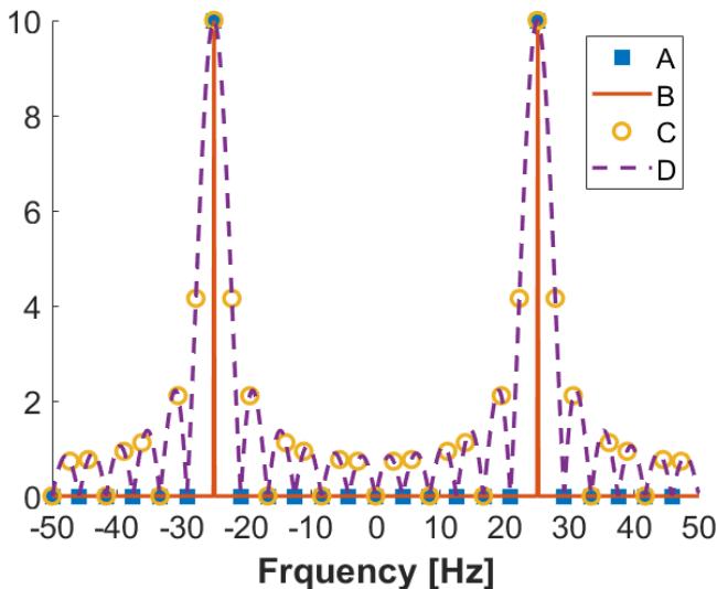
The infinitely-long discrete-time signal \(x[n]=20\cos(2\pi \frac{f}{f_s}n)\), with \(f=25\,\mathrm{Hz}\) and \(f_s=50\,\mathrm{Hz}\), is windowed with a rectangular window of length \(N\) to obtain the windowed signal \(\tilde x[n]\). In the plots below, the following Fourier transforms are shown:
- The Fourier Transform for Discrete time signals (FTD) of \(x[n]\)
- The FTD of \(\tilde x[n]\)
- The Discrete Fourier Transform (DFT) of \(\tilde x[n]\) calculated for \(N=24\) and zero padding of \(M=12\) samples
- The Discrete Fourier Transform (DFT) of \(\tilde x[n]\) calculated for \(N=24\) with no zero padding
Which of the following is the correct association?
- (a) 1B, 2D, 3A, 3C
- (b) 1B, 2D, 3C, 4A
- (c) 1C, 2A, 3D, 4B
- (d) 1D, 2B, 3C, 4A
Four objects, sharp → smeared → sampled. (1) Infinite cosine: two impulses at \(\pm 25\) Hz — infinitely sharp. So 1 = the sharpest plot (B). (2) Windowing to \(N\) multiplies by a rectangle = convolves with a sinc: the impulses fatten into main lobe + sidelobes. So 2 = the continuous smeared curve (D). (3–4) DFT samples that smeared curve: no padding = \(N\) sparse dots (A); zero-padding to \(N+M\) = denser dots on the same envelope (C). So 3 = C, 4 = A. Official: b) 1B, 2D, 3C, 4A. Option (a) has a typo (two "3"s) — free elimination. Note \(f=25\), \(f_s=50\): Nyquist is 25 Hz, the tone sits exactly there — that is why the plots alias symmetrically, and why the question works at all.
Spectral factorisation
Write \(P\) in \(\cos\theta\), replace \(\cos\theta=(z+z^{-1})/2\), factor \(P(z)=\sigma_i^2 L(z)L(z^{-1})\), put every pole and every zero of \(L\) inside the unit circle, scale so \(l[0]=1\). \(L(z^{-1})\) is max-phase and is the trap.
Resit · 24 Jan 2022 · 1d · 0.3 pt · one correct
Random signal \(x[n]\) has power spectral density
$$P_x(e^{j\theta})=\frac{\frac{17}{8}-\cos\theta}{\frac{25}{16}-\frac32\cos\theta},$$which is factorized as
$$P_x(e^{j\theta})=2\,\frac{1-\frac14 z-1+\frac14 z^{-1}}{1+\frac34 z+1+\frac34 z^{-1}}.$$Which of the following statements is true?
- a) The provided factorization does not represent the spectral factorization of signal \(x[n]\).
- b) The innovation filter is given by \(L(z^{-1})=(1-\frac14 z)/(1+\frac34 z)\).
- c) The innovation filter is given by \(L(z)=(1-\frac14 z^{-1})/(1+\frac34 z^{-1})\).
- d) The input variance is given by \(\sigma_i^2=1/2\).
What "innovation filter" means. Many filters share one \(|H|^2\); the innovation representation picks the unique minimum-phase one (all poles and zeros strictly inside \(|z|=1\), so system and inverse are both causal-stable) with \(l[0]=1\), scale in \(\sigma_i^2\). Kill: (b) \(L(z^{-1})\) runs on \(z^{+1}\) — anti-causal, maximum-phase by construction. (d) \(\sigma_i^2=1/2\): the printed gain is 2, and halving vs doubling is the reciprocal trap. Official: c, \(\sigma_i^2=2\). (The key notes a possible sign typo in the printed denominator — pick c anyway; the inside/outside pattern is unambiguous.)
Block 4 · which region is “decide \(\mathcal H_1\)”
Estimation outputs a number. Detection outputs a label. The two densities overlap, so every rule makes mistakes. You always write the likelihood ratio \(L=p(x\mid\mathcal H_1)/p(x\mid\mathcal H_0)\) and compare it to a threshold. After algebra you test a scalar. Which side of that scalar is \(\mathcal H_1\) is not always the right tail. That is the exam.
January 2019 published this ratio upside down. Later papers and SLT7 use \(p_1/p_0\). Write the standard ratio. Flag the 2019 key if you quote it.
Notation for this block
| Object | Symbol | Meaning |
|---|---|---|
| Hypotheses | \(\mathcal H_0\), \(\mathcal H_1\) | labels in the PDF — \(\mathcal H_0\) is not always "narrow" or "noise"; read the parameters |
| Likelihood ratio | \(L=p(\mathbf x\mid\mathcal H_1)/p(\mathbf x\mid\mathcal H_0)\) | scalar even if \(\mathbf x\) is a vector; decide \(\mathcal H_1\) iff \(L\ge\gamma\) |
| Sufficient statistic | \(T(\mathbf x)\), threshold \(\lambda'\) | after simplifying \(\ln L\): \(\lambda'\neq\gamma\), it absorbed constants, \(\sigma^2\), \(N\), \(\ln\gamma\) |
| False alarm | \(P_{\mathrm{FA}}=P(\text{decide }H_1\mid H_0)\) | \(\mathcal H_0\) density on the \(\mathcal H_1\) side — always under \(\mathcal H_0\), never "the overlap" |
| Detection / miss | \(P_D=P(\text{decide }H_1\mid H_1)\), \(P_M=1-P_D\) | \(\mathcal H_1\) density on the \(\mathcal H_1\) / \(\mathcal H_0\) side |
Method — five lines on the script. (1) Write \(L=p_1/p_0\), take \(\ln\), dump constants. (2) Isolate the statistic \(T\): re-derive the inequality direction — never memorise "right tail". Rule of thumb: \(\mathcal H_1\) wider/heavier → decide \(\mathcal H_1\) on large \(|x|\) (outer); \(\mathcal H_1\) narrower/faster → decide \(\mathcal H_1\) on small \(x\) (inner); mean shift → the shifted side. Multiplying by \(-1\) flips \(\gtrless\). (3) Sketch both densities, mark the threshold, shade \(P_{\mathrm{FA}}\) (\(H_0\) on the \(H_1\) side) and \(P_M\) (\(H_1\) on the \(H_0\) side). (4) NP: fix \(\lambda'\) from \(P_{\mathrm{FA}}=\alpha\) using only the \(\mathcal H_0\) law. Bayes 0–1: \(\gamma=P_0/P_1\) (equals 1 only for equal priors). (5) Compute the shaded areas: Gaussian → \(Q\)/erf; exponential/Laplace folded → \(e^{-\lambda\lambda'}\) (right side) or \(1-e^{-\lambda\lambda'}\) (left side); two-sided → double the one-sided tail.
H1 heavier tails or larger variance: decide H1 outside the dashed lines. False alarm is the H0 density on that outside. Miss is the H1 density in the middle.
H1 faster exponential or narrower Laplace: mass near zero, so decide H1 for small \(x\). The inequality on \(\sum T(x_n)\) flips when you multiply by −1. Hint on January 2020: “design so \(P_D>P_{\mathrm{FA}}\)” means take this left side.
Shade, always, after you know the region:
- \(P_{\mathrm{FA}}\): \(\mathcal H_0\) density on the \(\mathcal H_1\)-decision side.
- \(P_D\): \(\mathcal H_1\) density on the \(\mathcal H_1\)-decision side.
- \(P_M=1-P_D\): \(\mathcal H_1\) density on the \(\mathcal H_0\)-decision side.
False alarm is not “the overlap”. It is not under \(\mathcal H_1\).
Neyman–Pearson vs Bayes
Neyman–Pearson: maximise \(P_D\) at a fixed \(P_{\mathrm{FA}}=\alpha\). Set the threshold from the \(\mathcal H_0\) law only. The \(\mathcal H_1\) law is not used until you compute \(P_D\). Bayes, 0-1 costs: \(\gamma=P_0/P_1\). That is not \(\mathcal L=1\) unless the priors are equal.
ROC: \(P_D\) vs \(P_{\mathrm{FA}}\), upper triangle, through (0,0) and (1,1). Larger separation lifts the curve toward the top-left. If your curve sits in the lower triangle you used the CDF (left tail) instead of the complementary CDF, or you swapped the hypotheses.
Practice exam · 28 Oct 2021 · 1e · 0.5 pt · one correct
When plotting the receiver operating characteristic (ROC) curves, the common practice is to have the probability of detection \(P_d\) on the vertical axis and the probability of false alarm \(P_{fa}\) on the horizontal axis. In that case, the ROC curves should appear on the upper triangular part of the plot. Assume you are running simulations to generate ROC curves. The two hypotheses are
$$y[n]\sim\begin{cases}\mathcal N(0,\sigma^2)&\text{if }\mathcal H_0\\ \mathcal N(\mu,\sigma^2)&\text{if }\mathcal H_1\end{cases},\qquad\mu>0.$$If your curves appeared on the lower triangular part of the plot, which one of the following cannot be the reason?
- a) The variance of the null hypothesis \(\mathcal H_0\) is set too high.
- b) \(\mathcal H_0\) and \(\mathcal H_1\) are switched in the likelihood ratio.
- c) The cumulative probability density function is used to calculate \(P_d\).
- d) \(P_d\) and \(P_{fa}\) are switched.
What flips a ROC into the lower triangle. The ROC is \(P_D\) vs \(P_{\mathrm{FA}}\) as \(\gamma:0\to\infty\), through (0,0)–(1,1), concave, upper triangle for any sane detector. Three ways to land below the diagonal: (b) swap the hypotheses in the ratio (you detect \(H_0\)); (c) use the CDF instead of the survival function for \(P_D\) (you integrate the wrong tail); (d) swap the axes. All three invert the curve. (a) raising \(\sigma_0^2\) only blurs the two densities — the curve sags toward the diagonal, it never crosses it. Official: a ("cannot be the reason").
Four PDF pairs you will actually see
Retake · 21 Jan 2019 · 3b · 1.25 pt
Consider the two hypotheses
$$p(x)\sim\begin{cases}\mathcal N(0,1)&\mathcal H_0\\ \mathcal N(\mu_1,\sigma_1)&\mathcal H_1.\end{cases}$$The CDF is given as \(p(x\le X;\mu,\sigma)=\tfrac12\bigl[1+\mathrm{erf}((X-\mu)/(\sigma\sqrt 2))\bigr]\). Using the table for \(\mathrm{erf}(X/\sqrt 2)\) below, calculate \(P_d\) and \(P_{fa}\) for the listed thresholds \(X\), means \(\mu_1\) and standard deviations \(\sigma_1\).
| \(X\) | \(\mathrm{erf}\) |
|---|---|
| −3 | −0.997 |
| −2 | −0.954 |
| −1 | −0.683 |
| 0 | 0 |
| 1 | 0.683 |
| 2 | 0.954 |
| 3 | 0.997 |
| \(X\) | \(\mu_1\) | \(\sigma_1\) | \(P_d\) | \(P_{fa}\) |
|---|---|---|---|---|
| 1 | 1 | 1 | ||
| 1 | 3 | 1 | ||
| 1 | 3 | 2 | ||
| 2 | 3 | 1 |
How to read that erf table. The paper prints \(\mathrm{erf}(Z/\sqrt 2)\) against \(Z\) — and \(Z=(X-\mu)/\sigma\) is exactly the standardised distance, so look up \(Z\) directly, no \(\sqrt 2\) arithmetic. Right-tail probability: \(P(y>X)=\tfrac12[1-\mathrm{erf}]\). \(\mathrm{erf}\) is odd: \(\mathrm{erf}(-2)=-0.954\). Row by row: (1,1,1): threshold sits on the \(\mathcal H_1\) mean → \(P_d=0.5\) by symmetry, no table needed; \(P_{fa}\): \(Z=1\), erf \(0.683\), \(\tfrac12(1-0.683)=0.159\). (1,3,1): \(Z=(1-3)/1=-2\), erf \(-0.954\), \(P_d=\tfrac12(1+0.954)=0.977\); \(P_{fa}\) unchanged (\(\mathcal H_0\) did not move). (1,3,2): \(Z=(1-3)/2=-1\), \(P_d=\tfrac12(1+0.683)=0.842\) — wider \(\mathcal H_1\) leaks more mass left of the threshold, so \(P_d\) drops vs the previous row. (2,3,1): higher threshold, \(P_{fa}\): \(Z=2\), \(\tfrac12(1-0.954)=0.023\); \(P_d\): \(Z=(2-3)=-1\), \(0.842\). Official: 0.5/0.159; 0.977/0.159; 0.842/0.159; 0.842/0.023. Structural fact: \(P_{fa}\) uses only \(\mathcal H_0\) — it is 0.159 in the first three rows regardless of \(\mu_1,\sigma_1\). The erf table is printed on the paper; do not copy one onto the A4.
Written exam · 4 Nov 2019 · Q4 · 2 pt
Consider the binary hypothesis testing problem where the observed data \(x[0],x[1],\dots,x[n]\) consists of independent identically distributed samples and follows the PDFs
$$\mathcal H_0:\ x[n]\sim\mathcal N(0,\sigma_0^2),\qquad\mathcal H_1:\ x[n]\sim\mathcal N(0,\sigma_1^2),\qquad\sigma_1>\sigma_0.$$- (a) For a single sample, roughly plot the PDFs and mark the threshold for likelihood ratio \(\mathcal L(x[n])=1\). Write the equations for \(P_d\) and \(P_{fa}\) in terms of \(p(x[n];\mathcal H_1)\) and \(p(x[n];\mathcal H_0)\) (you don’t need to write the Gaussian PDF explicitly). [0.5 pt]
- (b) Calculate \(P_d\) and \(P_{fa}\) when \(\sigma_1=3\sigma_0\) and the likelihood ratio is chosen such that the threshold is \(x_{\mathrm{th}}=\sigma_1\). Use, for \(x\sim\mathcal N(0,\sigma^2)\): \(Pr(0\le x\le\sigma)=0.341\), \(Pr(\sigma\le x\le 2\sigma)=0.136\), \(Pr(2\sigma\le x\le 3\sigma)=0.021\). [0.5 pt]
- (c) Derive the log-likelihood ratio test that uses the observed data \(x[0],\dots,x[n]\), starting from \(\mathcal L(x)=p(\mathbf x;\mathcal H_1)/p(\mathbf x;\mathcal H_0)>\gamma\). [1 pt]
(a) Sketch + region. Both centred at 0; \(\mathcal H_1\) wider (\(\sigma_1>\sigma_0\)): tall narrow \(\mathcal H_0\) peak, short wide \(\mathcal H_1\). They cross at \(\pm x_{\mathrm{th}}\) (\(L=1\)). Far out, the wide density wins, so decide \(\mathcal H_1\) outside the lines (two outer tails). Write the equations with the densities, not the Gaussian formula (the paper says so): \(P_D=2\int_{x_{\mathrm{th}}}^\infty p(x\mid\mathcal H_1)dx\), \(P_{fa}=2\int_{x_{\mathrm{th}}}^\infty p(x\mid\mathcal H_0)dx\). The factor 2 is the two sides — forgetting it is the standard half-mark loss.
(b) Numbers — convert the threshold to each hypothesis's own units. \(x_{\mathrm{th}}=\sigma_1=3\sigma_0\). Under \(\mathcal H_1\) that is one own-sd out: \(P_D=2(0.5-0.341)=0.318\). Under \(\mathcal H_0\) it is three own-sd out: stack the printed bands \(0.341+0.136+0.021=0.498\), so \(P_{fa}=2(0.5-0.498)=0.004\). Official. Rule: always express the threshold in the units of the density you integrate — "3 sd out" vs "1 sd out" is the whole computation.
(c) Log-LRT — why squares. IID product, \(\ln\), group: the \(x_n^2\) terms survive (variances differ, means don't), the \(x_n\) terms never appear. Coefficient of \(\sum x^2\): \(1/\sigma_0^2-1/\sigma_1^2>0\) (since \(\sigma_1>\sigma_0\)) so decide \(\mathcal H_1\) when \(\sum x[n]^2\) is large. Energy detector, not a mean detector. (The with-answers key drops the squares — typesetting bug; the oldexams key has them.) If \(\sigma_1<\sigma_0\) the coefficient would flip and \(\mathcal H_1\) would be the inner region — same derivation, opposite side.
Written exam · 20 Jan 2020 · Q5 · 2.5 pt
Consider the binary hypothesis testing problem where the observed data \(x[0],x[1],\dots,x[n]\) consists of independent identically distributed samples and follows the exponential PDFs
$$\mathcal H_0:\ x[n]\sim\lambda_0 e^{-\lambda_0 x},\qquad\mathcal H_1:\ x[n]\sim\lambda_1 e^{-\lambda_1 x},$$where \(x\ge 0\), \(\lambda_1>\lambda_0>0\).
- (a) For a single sample, roughly plot the PDFs for \(\lambda_1=2\) and \(\lambda_0=0.1\). Calculate and mark the threshold \(x_{\mathrm{th}}\) for likelihood ratio \(\mathcal L(x_{\mathrm{th}})=1\). Write the equations for \(P_d\) and \(P_{fa}\) in terms of \(\lambda_0\), \(\lambda_1\) and \(x_{\mathrm{th}}\). [0.75 pt] Hint: the CDF is \(P(x<x_{\mathrm{th}})=1-e^{-\lambda x}\). Design your test such that \(P_d>P_{fa}\).
- (b) Given \(\lambda_0=0.1\), find \(\lambda_1\) that gives \(P_d=0.9\) when \(P_{fa}=0.1\). [0.5 pt]
- (c) Plot the ROC for that \(\lambda_1\), using \(P_{fa}=0.5\) and \(P_{fa}=0.9\) as reference points. Roughly sketch two more curves for \(\lambda_1\) increased and \(\lambda_1\) decreased. [1.25 pt]
(a) Sketch first, then the threshold. Two exponentials on \(x\ge 0\), each starting at its rate: \(\mathcal H_1\) (\(\lambda_1=2\)) starts high and dies fast; \(\mathcal H_0\) (\(\lambda_0=0.1\)) starts low and dies slowly. Sketch rule: height at 0 = rate, decay speed = rate — the faster one starts taller. They cross once. Set \(L(x_{\mathrm{th}})=1\): \((\lambda_1/\lambda_0)e^{-(\lambda_1-\lambda_0)x_{\mathrm{th}}}=1\), so \(x_{\mathrm{th}}=\ln(\lambda_1/\lambda_0)/(\lambda_1-\lambda_0)=\ln 20/1.9\approx 1.58\). Official.
Which side is \(\mathcal H_1\)? \(L(x)\) is a decreasing exponential in \(x\) (since \(\lambda_1>\lambda_0\)), so \(L>1\) iff \(x<x_{\mathrm{th}}\): decide \(\mathcal H_1\) for small \(x\), left of the line. That is what the hint ("design so \(P_D>P_{fa}\)") means — the other side would give \(P_D<P_{fa}\) (below the ROC diagonal). Shade: \(P_D\) is \(\mathcal H_1\) on \((0,x_{\mathrm{th}})\), \(P_{fa}\) is \(\mathcal H_0\) on \((0,x_{\mathrm{th}})\). With the printed CDF: \(P_D=1-e^{-\lambda_1 x_{\mathrm{th}}}\), \(P_{fa}=1-e^{-\lambda_0 x_{\mathrm{th}}}\).
(b) Operating point, two inversions. NP logic: the threshold comes from \(\mathcal H_0\) alone. Fix \(P_{fa}=0.1\): \(1-e^{-0.1x_{\mathrm{th}}}=0.1\), so \(x_{\mathrm{th}}=-10\ln 0.9\approx 1.05\). Then demand \(P_D=0.9\) at that threshold: \(1-e^{-\lambda_1\cdot 1.05}=0.9\), so \(\lambda_1=\ln 10/1.05\approx 2.19\). Official. Order matters: threshold from \(H_0\), performance from \(H_1\) — never the reverse.
(c) ROC — parametrize by the threshold. Each \(x_{\mathrm{th}}\) is one \((P_{fa},P_D)\) point: \(x_{\mathrm{th}}\to 0\) gives (1,1), \(x_{\mathrm{th}}\to\infty\) gives (0,0). The paper's \(P_{fa}=0.5\) (\(x_{\mathrm{th}}=-10\ln 0.5\approx 6.93\), \(P_D\approx 1\)) and \(P_{fa}=0.9\) (\(x_{\mathrm{th}}\approx 23\), \(P_D\approx 1\)) are two dots on the same curve — compute, mark, join through (0,0)–(1,1). Larger \(\lambda_1\) = easier separation = harder bow toward top-left; smaller = sag toward the diagonal. Sketch three curves, label which is which. Curve below the diagonal means you integrated the wrong tail — flip.
Resit · 24 Jan 2022 · 4a–c
4a. Which of the following statements about the matched filter is true? [0.3 pt]
- (a) The signal-to-noise ratio at the output of the matched filter is maximized.
- (b) The matched filter can be implemented as a FIR filter with impulse response \(h[n]=s[n]\).
- (c) The matched filter can only be applied for uncorrelated noise samples.
4b. Consider hypotheses [0.7 pt]
$$p_Y(y\mid\mathcal H_0)=\frac{1}{\sqrt{2\pi}}e^{-y^2/2},\qquad p_Y(y\mid\mathcal H_1)=\frac14 e^{-|y|/2}.$$Provide a sketch for the two PDFs and indicate the probability of false alarm and missed detection for a likelihood test with \(\gamma=1\).
4c. Compute \(P_D\) and \(P_{\mathrm{FA}}\) at that threshold. The 2022 paper prints a \(Q\)-table; they use \(Q(1.59)=0.0559\). [1.0 pt]
4a — one line each. Official: a. Matched filter = SNR-optimal linear filter (Cauchy–Schwarz: \((h^\top s)^2\le(h^\top h)(s^\top s)\), equality iff \(h\propto s\) — that proportionality is the filter). (b) is the correlate-vs-convolve trap: filtering convolves, so the FIR form time-reverses, \(h[n]=s[N-1-n]\), sampled at \(n=N-1\); \(h[n]=s[n]\) only correlates. (c) is false — coloured noise just needs a whitening front-end first; "only uncorrelated" confuses the textbook example with the definition.
4b — sketch + shade. \(\mathcal H_0=\mathcal N(0,1)\): tall narrow bell. \(\mathcal H_1=\frac14e^{-|y|/2}\): shorter peak, heavier tails (exponential tails beat Gaussian tails far out). So \(\mathcal H_1\) = outer tails, thresholds at \(\pm y_{\mathrm{th}}\) where \(L=1\). Shade with the rule: \(P_M\) is \(\mathcal H_1\) truth on the \(\mathcal H_0\) side = the centre of the Laplace (between the lines); \(P_{fa}\) is \(\mathcal H_0\) truth on the \(\mathcal H_1\) side = the Gaussian tails (outside the lines). Say the rule out loud before shading — putting one area on the wrong density is the standard half-mark loss.
4c — numbers, both doubled. \(L=1\) gives \(-|y|+y^2=2\ln 4-\ln(2\pi)\), so \(y_{\mathrm{th}}=\pm 1.5884\). Laplace tail (one side, times 2 by evenness): \(P_D=e^{-1.5884/2}=0.4519\). Gaussian (Q-table printed, \(Q(1.59)=0.0559\), times 2): \(P_{fa}=2\times 0.0559=0.1118\). Official. Two-sided test: every tail count doubles. Forgetting one factor of 2 is the arithmetic trap.
Final exam · 7 Nov 2022 · 4c–d · no official key
Under the two hypotheses a single observation \(x\) admits a zero-mean Laplacian distribution, but with different variances:
$$p(x;\mathcal H_0)=\tfrac12 e^{-|x|},\qquad p(x;\mathcal H_1)=e^{-2|x|}.$$Assume the \(N\) observations are iid. 4c. Show that the likelihood ratio test takes the form
$$\sum_{n=0}^{N-1}|x_n|\;\underset{\mathcal H_1}{\overset{\mathcal H_0}{\gtrless}}\;\gamma'$$and determine \(\gamma'\). Hint: pay special attention to the inequality. [0.5 pt]
4d. For \(N=1\), set \(Y=|X|\), so \(p(y;\mathcal H_0)=e^{-y}\), \(p(y;\mathcal H_1)=2e^{-2y}\), and \(y\gtrless_{\mathcal H_1}^{\mathcal H_0}\gamma'\). The two densities are plotted below. Indicate \(P_{\mathrm{FA}}\) and \(P_M\) for \(\gamma'=1\). [0.25 pt]
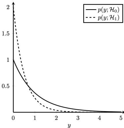
4c — the inequality flip, slowly. IID, so the joint ratio is a product: L = 2^N exp(-sum|x_n|). Take logs: N ln2 - sum|x_n| compared against ln(gamma), H1 on top. Now move the sum to the left by multiplying by -1 — the inequality flips, and H1 ends up at the bottom: decide H0 when the sum of absolute values is large. Why: H1 is the narrower Laplace (rate 2 vs 1 — taller peak, faster decay), so large |x| favours H0. Threshold: N ln2 - ln(gamma) (tagged derived — no official Nov22 key). Writing the unflipped inequality is the 0.5-pt loss; the hint on the paper says pay special attention to the inequality, and this is what it means.
4d — shade on the folded plot. N=1, Y=|X|: H0 density exp(-y), H1 density 2exp(-2y), y>0. At threshold 1, decide H1 for y<1 (left of the line — not the usual right tail). P_FA: H0 density on (0,1), under the solid curve. P_M: H1 density on (1, infinity), under the dashed curve. If you shade right-tails by habit you shade exactly the complements. Look at the photo: solid starts at 1, dashed at 2 — at y=0, H1 is twice as tall, so the left region is H1's.
Marking keys
Use these after you sit the paper. no official key means there is no published letter. derived is computed here, never a published letter.
Jan 2019 retake · 21 Jan · 18.00–21.00
Four exercises. Q1 = 4 MC × 0.5, one or two correct, extra wrong −0.25. Q3 is SLT7 7.1. Q4 is 2-tap Wiener: legacy, not a 2026 model.
| Q | what it is | official |
|---|---|---|
| 1a | discrete / continuous | B, C dice count; phone number |
| 1b | which formula is MLE | D \(\hat\theta=\arg\max p(x\mid\theta)\) |
| 1c | nonparametric SE | A, C (Bartlett bias up; BT consistent) |
| 1d | linear models | C, D. MA ACF has \(2Q+1\) lags, not \(Q\). |
| 2a | exponential MLE | \(\hat\lambda_{\mathrm{ML}}=N/\sum x_i\) |
| 2b | MMSE, Unif\([0,2]\) | one-sample formula despite \(N\) in 2a. See errata. |
| 2c | MAP, same prior | \(N/\sum x_i\) (= MLE). Key skips the projection onto \([0,2]\). |
| 3a | LRT | inverted \(\mathcal L=p(\mathcal H_0)/p(\mathcal H_1)\). See errata. |
| 3b | erf table | \((P_D,P_{\mathrm{FA}})\): 0.5 / 0.159; 0.977 / 0.159; 0.842 / 0.159; 0.842 / 0.023 |
| 4a | Wiener \(H=1\) | \(\mathbf w=(1,2)^\top\), \(J_{\min}=0\) |
| 4b | Wiener \(H=1-2z^{-1}\) | \(\mathbf w=(-1,0)^\top\), \(J=\tfrac43\) |
Nov 2019 · 4 Nov · 13.30–16.30
Four exercises. Two keys (exam-with-answers + oldexams). Sit this for the correlogram / AR(2) pair and the energy detector.
| Q | what it is | official |
|---|---|---|
| 1a | finite-record \(r_{xy}\) | exam-with-answers B; oldexams no option is correct (B lagged). See errata. |
| 1b | T/F five statements | F F T T F. A dropped as ambiguous. E is AR prediction, not MA. |
| 1c | fill nonparametric table | Key fully fills periodogram only: \(\frac1N|\sum x e^{-jn\theta}|^2\); bias = FT of biased ACF; var \(\propto P^2\). |
| 2a | correlogram | \(1+1.4\cos\theta+\cos 2\theta+0.6\cos 3\theta\). Can go negative. |
| 2b | AR(2) | \(0.5089\big/|1-0.6863 e^{-j\theta}-0.0196 e^{-j2\theta}|^2\). Strictly positive. |
| 3a | Rayleigh MLE | \(\hat\theta=\sqrt{(1/(2N))\sum x^2[n]}\) |
| 3b | CRLB | key wrote \(\hat\theta^2/(4N)\). Bound is \(\theta^2/(4N)\). |
| 3c | MAP, exp prior | implicit cubic in \(\theta\). Depends on \(\lambda\). |
| 4a | variance detector, shade | H1 = tails. \(P_D=2\int_{x_{\mathrm{th}}}^\infty p(x;\mathcal H_1)\,dx\) |
| 4b | numbers | \(P_D=0.318\), \(P_{\mathrm{FA}}=0.004\) |
| 4c | log-LRT | energy detector, formula above |
Jan 2020 · 20 Jan · 18.00–21.00
Five exercises. MC exactly one; options are unlettered bullets, key uses A/B/C/D = 1st/2nd/3rd/4th.
| Q | what it is | official |
|---|---|---|
| 1a | valid ACF plots | A only \(r_B\). \(r_C\) even with \(r[0]\) max but \(P(\pi)<0\). |
| 1b | Welch / WOSA | D overlap, same \(K\): var larger than Bartlett, still below the periodogram |
| 1c | windowing | C wider main lobe, worse resolution |
| 1d | expected value | B mean over an infinite number of observations |
| 2a | paint, total P | \(P[A]=0.819\) |
| 2b | paint, posterior | \(P[M_3\mid A]=0.18\) |
| 3a | correlogram | \(\tfrac4{105}\cos\theta+\tfrac1{21}\) |
| 3b | MA(1) | identical to 3a. Min-phase \(b=\tfrac12\), not \(b=2\). |
| 4a | which estimator | least squares (no noise PDF) |
| 4b | \(\phi\) known | \(\hat A_{\mathrm{ls}}=\sum x[n]e^{\phi n}/\sum e^{2\phi n}\) |
| 4c | both unknown | \(J=\sum(x[n]-A e^{\phi n})^2\). Nonlinear. |
| 4d | Gauss–Newton | key printed Newton on \(J\): \(\theta_{k+1}=\theta_k-H^{-1}\nabla J\) |
| 5a | two exponentials | \(x_{\mathrm{th}}=1.58\). H1 = small \(x\). \(P_D=1-e^{-\lambda_1 x_{\mathrm{th}}}\) |
| 5b | operating point | \(x_{\mathrm{th}}=1.05\), \(\lambda_1=2.19\) |
| 5c | ROC | larger \(\lambda_1\) ⇒ steeper (closer to top-left) |
Jan 2020 resit · 24 Jan · same exam as Jan 2022 resit
No separate question PDF for 2020. Recover from Resit 2020 solutions. Letters below are those on the 2022 paper. 2f–h is SLT4 2025–26 4.3.
| Q | what it is | official |
|---|---|---|
| 1a | employees / experience | 0.26 (c) |
| 1b | pixel / picture | b each picture is a realization = a random signal |
| 1c | dice ensemble | b ergodic in mean and variance |
| 1d | factorisation | c \(L(z)=(1-\tfrac14 z^{-1})/(1+\tfrac34 z^{-1})\), \(\sigma_i^2=2\). See errata. |
| 2a | CRLB MC | b iid ⇒ CRLB decreases linearly with \(N\) |
| 2b | MLE MC | c invariance |
| 2c | LS MC | a some NL-LS separate. Key: “no longer part of the content.” |
| 2d | Bayesian MC | b MMSE = mean of the posterior |
| 2e | regularity | cannot. Support depends on \(\theta\). |
| 2f | BPSK posteriors | softmax of \(\mathcal N(\pm 1,\sigma^2)\) |
| 2g | MMSE | \(\tanh(y/\sigma^2)\) |
| 2h | MAP | \(\mathrm{sign}(y)\) |
| 3a | FTD / DFT plot | B = 1B, 2D, 3C, 4A |
| 3b | MA(2) | \(b=r[2]=\tfrac14\), \(a=-\tfrac34\) |
| 3c | correlogram | \(\tfrac{13}8-\tfrac{15}8\cos\theta+\tfrac12\cos 2\theta\) |
| 3d | AR(1) | \(a_1=\tfrac{15}{26}\), \(\sigma_i^2=\tfrac{451}{416}\) |
| 4a | matched filter | a output SNR maximised |
| 4b | Gauss vs Laplace, shade | H1 = tails. \(P_M\) = centre of H1; \(P_{\mathrm{FA}}\) = H0 tails. |
| 4c | numbers | \(y_{\mathrm{th}}=\pm 1.5884\), \(P_D=0.4519\), \(P_{\mathrm{FA}}=0.1118\) |
Practice · 28 Oct 2021
Part 1: 6 MC × 0.5, PMFs printed. Parts 2–4 open. Q3 is SLT6 2025–26 6.2. 1f has no worked slide.
| Q | what it is | official |
|---|---|---|
| 1a | virus Bayes | b) 37% |
| 1b | cov vs corr | d) all of the above |
| 1c | \(E[X]\) discrete | b weighted average over outcomes |
| 1d | binomial | d) 0.2936 |
| 1e | ROC lower triangle | a “H0 variance too high” cannot flip the ROC |
| 1f | t-statistic | no official key · derived c is false (small \(t\) is more consistent with H0) |
| 2a | CRLB equality → PDF | they stop at the law of \(\bar x\), not the full \(N\)-sample Gaussian |
| 2b | Rayleigh \(\theta=\sigma^2\) | \(\hat\theta=(1/(2N))\sum x^2[n]\) (no square root) |
| 3a | ARMA(1,1) ACF | \(\rho[0]=\tfrac{28}{27}\), \(\rho[1]=-\tfrac4{27}\), then AR tail. Fallback \(\rho[1]=+5/27\) is the wrong sign on purpose. |
| 3b | AR(1) | \(a_1=\tfrac17\), \(\sigma_i^2=\tfrac{64}{63}\). \(P(0)=0.78\), \(P(\pi)=1.38\) (high-pass). |
| 3c | MA(1) correlogram | \(\tfrac{28}{27}-\tfrac8{27}\cos\theta\) |
| 4a | erf + ROC | \(P_{\mathrm{fa}}(0)=0.5\), \(P_{\mathrm{fa}}(1)=0.1585\). \(\mu=2\) ROC strictly above \(\mu=1\). |
| 4b | log-LRT | identical to Nov 2019 4c |
Jan 2022 resit · 24 Jan · 18.00–21.00
Questions = January 2020 resit. Grade with the table above. Cover says answers on paper. 4c uses \(Q(1.59)=0.0559\). 1a options 0.24 / 0.25 / 0.26 / 0.28. 3a option (a) has a typo (two “3”s); official (b).
Nov 2022 · 7 Nov · 13.30–16.30 no official key
Split on cover 1.5 / 2.75 / 3 / 2.75. Closest to the current format. Every cell below is derived or a lecture fact. None is a published letter.
| Q | what it is | answer |
|---|---|---|
| 1a | followed the course | derived \(0.65\cdot 0.75+0.35\cdot 0.4=0.6275\approx 0.63\) (c) |
| 1b | joint → marginal | derived \(p_X(0)=13/24\), \(p_X(1)=11/24\) (b) |
| 1c | RNG / ergodic | derived ensemble mean 0; time-variance \(A^2/3\) varies across realizations ⇒ not fully ergodic. Do not guess a letter. |
| 1d | factorisation · 0.75 | derived \(L(z)=1/(1-\tfrac13 z^{-1})\), \(\sigma_i^2=\tfrac23\) |
| 2a | Fisher MC | derived (a) \(N\) iid ⇒ \(\mathcal I=N i(\theta)\) |
| 2b | MLE MC | derived (c) asymptotically unbiased |
| 2c | Bayes MC | derived (b) Bayes risk definition. Uniform cost ⇒ MAP, not MMSE. |
| 2d | angle MLE · 0.5 | derived \(\hat\theta_{\mathrm{ML}}=\mathrm{atan2}(x_2,x_1)\) |
| 2e | Fisher · 0.5 | derived \(\mathcal I(\theta)=A^2/\sigma^2\) |
| 2f | MMSE · 0.5 | derived Gamma(2, \(x+a\)), mean \(2/(x+a)\) |
| 2g | MAP · 0.5 | derived mode \(1/(x+a)\) |
| 3a | Bartlett vs WOSA | derived (a) Bartlett var \(\propto 1/K\), bias increases. Overlap ⇒ not \(1/K\). |
| 3b | window / zeropad | lecture fact: main lobe = resolution, side lobes = leakage. Do not guess a letter. |
| 3c | what process · 0.15 | derived ARMA(1,1), \(a_1=-\tfrac34\), \(b_1=-1\) |
| 3d | \(P_x\) · 0.35 | derived \(\frac78 |1-e^{-j\theta}|^2\big/|1-\tfrac34 e^{-j\theta}|^2\) |
| 3e | ACF · 0.5 | derived \(r[0]=1\), \(r[1]=-\tfrac18\), then \(r[\tau]=\tfrac34 r[\tau-1]\) for \(|\tau|>1\) |
| 3f | AR(1) · 0.75 | derived \(a_1=\tfrac18\), \(\sigma_i^2=\tfrac{63}{64}\) |
| 3g | MA(1) · 0.75 | derived \(1-\tfrac14\cos\theta\) |
| 4a | confusion-matrix labels | derived (a) 1=TN, 2=FN/miss, 3=FP/FA, 4=TP |
| 4b | Neyman–Pearson | derived (b) fixed \(P_{\mathrm{FA}}\), max \(P_D\) |
| 4c | two Laplaces · 0.5 | derived \(\sum|x_n|\gtrless_{\mathcal H_1}^{\mathcal H_0}\gamma'\), H1 = small sum. \(\gamma'=N\ln 2-\ln\gamma\). |
| 4d | shade · 0.25 | derived H1 for \(y<1\). \(P_{\mathrm{FA}}\) = H0 on \((0,1)\); \(P_M\) = H1 on \((1,\infty)\). |
| 4e | NP point · 0.5 | derived \(P_{\mathrm{FA}}=0.1\Rightarrow\gamma'=-\ln 0.9\approx 0.105\), \(P_D=0.19\) |
| 4f | Bayes threshold · 0.5 | derived \(\gamma''=\ln 3\approx 1.099\) |
| 4g | Bayes errors · 0.5 | derived \(P_M=\tfrac19\), \(P_{\mathrm{FA}}=\tfrac23\) |
Key errata
These are the published keys being wrong, not you.
Jan 2019 3a: the published LRT is inverted, \(\mathcal L=p(\mathcal H_0)/p(\mathcal H_1)\). Later papers use \(p_1/p_0\). Write the standard ratio; flag the key if you quote 2019.
Nov 2019 1a: exam-with-answers says B; oldexams says no option is correct (B is the sequence lagged / reversed). Direct \(r_{xy}[\tau]=\frac1N\sum x[n]y[n+\tau]\) matches shifted-B. Prefer oldexams.
Jan 2019 2b: published MMSE is the one-sample formula despite \(N\) in 2a. The \(N\)-sample version is a truncated \(\mathrm{Gamma}(N+1,S)\), \(S=\sum x_i\).
Nov 2019 3b: the key writes \(\mathrm{VAR}(\hat\theta)\ge\hat\theta^2/(4N)\). It plugged the estimate. The bound is \(\theta^2/(4N)\).
Jan 2019 2c: MAP omits the projection onto \([0,2]\). Uniform prior is flat on \((0,2)\), so MAP = MLE only if the unconstrained MLE sits inside; otherwise \(\hat\lambda=2\).
Jan 2022 resit 1d: the key notes a possible sign typo in the printed factorisation denominator. Official letter is still c, \(\sigma_i^2=2\) not \(1/2\). \(L(z^{-1})\) is max-phase.
5CTA0 Q1 2026–27 · from the course reader, lectures and official keys.